《Quantum Chemistry》章末总结9

隔了有半年了才接着写下一章XD，本章是多电子原子，算是量子化学正式开场了。

Chapter 9 Many-Electron Atoms

Helium is our first multielectron system, and although the helium atom may seem to be of minimal interest to chemists, we will discuss it in detail in this chapter because the solution of the helium atom illustrates the techniques used for more complex atoms.

Then, after discussing electron spin and the Pauli exclusion principle, we will discuss the Hartree-Fock theory of many-electron atoms.

Finally, we will discuss the term symbols of atoms and ions and how they are used to label electronic states.

9.1 Atomic and Molecular Calculations Are Expressed in Atomic Units

We will apply both perturbation theory and the variational method to a helium atom, but before doing so, we will introduce a system of units, called atomic units, that is widely used in atomic and molecular calculations to simplify the equations.

Property	Atomic unit	SI equivalent
Mass	Mass of an electron,$m_e$	$9.1094\times10^{-31}\ \rm kg$
Charge	Charge on a proton,$e$	$1.6022\times10^{-19}\ \rm C$
Angular momentum	Planck constant divided by 2π,$\hbar$	$1.0546\times 10^{-34}\ \rm J\cdot s$
Length	Bohr radius,$a_0=\frac {4\pi\epsilon_0\hbar^2}{m_ee^2}$	$5.2918\times 10^{-11}\ \rm m$
Energy	$\frac {m_ee^4}{14\pi^2\epsilon_0^2\hbar^2} = \frac {e^2}{4\pi\epsilon_0a_0} = E_h$	$4.3597\times 10^{-18}\ \rm J$
Permittivity	$\kappa_0 = 4\pi\epsilon_0$	$1.1127\times 10^{-10}\ \rm C^2\cdot J^{-1}\cdot m^{-1}$

（ 第一节就是讲原子单位，通过约定一些常量来简化算式。 ）

9.2 Both Perturbation Theory and the Variational Method Can Yield Good Results for a Helium Atom

We applied first-order perturbation theory to a helium atom in Section 8.5 and found
that the first-order correction to the energy is $5Z/8E_h$.The first-order perturbation theory gives a result that is approximately 5% in error.

Scheer and Knight calculated the energy through many orders of perturbation theory and found that $E=-2.9037E_h$, in good agreement with the experimental value of $-2.9033E_h$.

We also used the variational method to calculate the ground-state energy of a helium
atom in Section 8. 1, and $E_{min}=-2.84766E_h$.

The agreement we have found between first-order perturbation theory or our simple
variational approximation and the experimental value of the energy may appear to be
quite good, but let’s examine this agreement more closely. The ionization energy (IE)
of a helium atom is given by:

$IE = E_{He^{+}} - E_{He}$

The energy of $He^{+}$ is $-2E_h$, so we have:

$\begin{aligned} IE &= -2 + \frac {11}{4} = 0.75E_h \quad (\rm first-order\ perturbation\ theory)\\[3mm] or \\[3mm] &= -2 + \left(\frac {27}{16} \right) = 0.8477E_h \quad (\rm our\ variational\ result) \end{aligned}$

whereas the experimental value of the ionization energy is $0.9033E_h$. Even our variational result, with its 6% discrepancy with the experimental total energy, is not too satisfactory.

One approach is the following. The trial function assumes that both electrons have the same effective nuclear charge. This may be so in some average sense, but it will not be true at all times because there will be instants of time where one electron is far from the nucleus and the other close to it, and so the effective nuclear charges will not be the same.

We can account for this by using two variational parameters, $\zeta_1$ and $\zeta_2$. In order to treat the two electrons on an equal footing, we write $\psi(\bold {r_1}, \bold {r_2})$ as

$\psi(\bold {r_1}, \bold {r_2}) = N(e^{-\zeta_1r_1} e^{-\zeta_2r_2} + e^{-\zeta_2r_1} e^{-\zeta_1r_2})$

When $E(\zeta_1, \zeta_2)$ is minimized with respect to $\zeta_1$ and $\zeta_2$, we find that $E=-2.87566E_h$, which is a significant improvement over our simple variational treatment. The ionization energy comes out to be $0.8757E_h$.

we can do better yet. Because a suitable trial function may be almost any convenient function (that satisfies the boundary conditions), we are not restricted to using 1s hydrogen-like orbitals as we have done up to now. For example, we could use a linear combination of a 1s orbital and a 2s orbital and write:

$\psi(\bold {r_1}, \bold {r_2}) = \phi(\bold {r_1})\phi(\bold {r_2})$

where $\phi(r) = N[c_1e^{\zeta r}+c_2(2-r)e^{-\zeta r/2}]$ and $N$ is a normalization constant.

However, rather than using hydrogen-like orbitals, it’s customary to use a set of functions that were introduced by the American physicist John Slater in the 1930s. These functions, which are called Slaler orbitals, are of the form

$S_{nlm_l}(r, \theta, \phi) = N_{nl} r^{n-1} e^{-\zeta r} Y_l^{m_l}(\theta, \phi)$

where $N_{nl}$ is a normalization constant and the $Y_m^{m_l}(\theta, \phi)$ are the spherical harmonics. Note that the radial parts of Slater orbitals do not have nodes like hydrogen atomic orbitals do.

As we include more and more Slater orbitals, we reach a limit that is both practical
and theoretical. In this limit, $E = -2.8617E_h$ and the ionization energy is $0.8617E_h$. This limiting value is the best value of the energy that can be obtained using a trial function of the form of a product of one-electron wave functions. This limit is called the Hartree-Fock limit.

（ 由于试验函数可以任选，因此选择合适的试验函数是取得更高精度结果的一个重要因素，Hartree-Fock法的优点在于其不仅计算相对简单，而且与物理情景有着很好的对应。 ）

9.3 Hartree-Fock Equations Are Solved by a Self-Consistent Procedure

The starting point of the Hartree-Fock procedure for a helium atom is to write the two-electron wave function as a product of orbitals:

$\Psi(\bold r_1, \bold r_2) = \psi(\bold r_1) \psi(\bold r_2)$

We can also interpret this probability distribution classically as a charge density, and so we can say that the potential energy that electron 1 experiences at the point $\bold r_1$ due to electron 2 is

$V_1^{eff}(\bold r_1) = \int \psi^*(\bold r_2) \frac 1{\bold r_{12}} \psi(\bold r_2) d\bold r_2$

where the superscript “eff” emphasizes that $V_1^{eff}(\bold r_1)$ is an effective, or average, potential.

We now define an effective one-electron Hamiltonian operator by:

$\hat H_1^{eff}(\bold r_1) = -\frac 12 \nabla_1^2 - \frac 2{r_1} + V_1^{eff}(\bold r_1)$

The first term represents the kinetic energy of the electron, the second term represents its potential energy due to the electron-nucleus interaction, and the third term represents the potential energy due to its interaction with the other electron. The Schrödinger equation corresponding to this effective Hamiltonian operator is

$\hat H_1^{eff}(\bold r_1)\psi(\bold r_1) = \epsilon_1 \psi(\bold r_1)$

Because $\psi(\bold r_1)$ and $\psi(\bold r_2)$ have the same functional form, we need to consider only one equation. The equation above is the Hartree-Fock equation for a helium atom.

（ 上面是通过物理情景推导出的Hartree-Fock方程，接下来用变分法导出。 ）

Considering that:

$E = \int \int d\bold r_1 d\bold r_2 \psi^*(\bold r_1) \psi^*(\bold r_2)\hat H \psi(\bold r_1)\psi(\bold r_2)$

we have assumed that the $\psi$'s are normalized. If we substitute the expression of $\hat H$ into the equation, than we find

$E = I_1 + I_2 + J_{11}$

and

$J_{11} = \int \int d\bold r_1 d\bold r_2 \psi^*(\bold r_1) \psi^*(\bold r_2) \frac {1}{\bold r_{12}} \psi(\bold r_1)\psi(\bold r_2)$

The integral $J_{11}$ here is called a Coulomb integral because it has a classical interpretation of the interaction between two charge distributions.

We can obtain the Hartree-Fock equation by minimizing E with respect to $\psi$.

Recall that $V_1^{eff}(\bold r_1)$ depends upon $\psi(\bold r_2)$. Thus, we must know the solution before we even know $H_1^{eff}(\bold r_1)$. The method of solving an equation like that is by the self-consistent field method.

We first guess the form of $\psi(r)$. We next use $\psi(r)$ to evaluate $V_1^{eff}(\bold r_1)$ and then solve for a new $\psi(r_1)$. Usually, after one cycle like this, the $\psi(r)$ that is used as input and the $\psi(r_1)$ obtained as output differ. We then use this new $\psi(r)$ as input by calculating $V_1^{eff}(\bold r_1)$ with this new $\psi(r)$ and then solve equation for a newer $\psi(r_1)$. This cyclic process is continued until the $\psi(r)$ used as input and the $\psi(r)$ obtained from the equation are sufficiently close, or are self-consistent.

（ 自洽场方法的精髓就是通过不断地将前一轮计算结果作为新的输入，然后运算得到新的结果，再次作为输入，不断循环迭代，直到误差足够小，精度足够高时，即迭代完成，满足了自洽。 ）

The eigenvalue $\epsilon_1$ has the following physical significance.

$\int d\bold r_1 \psi^*(\bold r_1) \hat H_1^{eff}(\bold r_1) \psi(\bold r_1) = \epsilon_1 = I_1 + J_{11}$

We first note that the total energy of a helium atom is not the sum of its orbital energies because

$\epsilon_1 + \epsilon_2 = (I_1 + J_{11})+(I_2 + J_{11}) \neq E$

and

$\epsilon_1 = E - I_2$

This equation suggests that the orbital energy $\epsilon_1$ is an approximation to the ionizaton energy of a helium atom or that

$IE \approx -\epsilon_1$

It’s known as Koopmans’s approximation. Even within the Hartree-Fock approximation, Koopmans’s approximation assumes that the same orbitals can be used to calculate the energy of the neutral atom and the energy of the ion.

Because $\Psi(\bold r_1, \bold r_2) = \psi(\bold r_1)\psi(\bold r_2)$, the two electrons are aassumed to interact only through some average, or effective, potential. We say, then, that the electrons are uncorrelated, and we define a correlation energy ($E_{corr}$) by the equation

$E_{corr} = E_{exact} - E_{HF}$

（ HF方法的极限指和真实值的差称为相关能，主要是由于忽略了库伦作用产生的。 ）

In practice, when carrying out a Hartree- Fock calculation, we use linear combinations of Slater orbitals for $\psi(r)$, varying the coefficients for each Slater orbital until convergence is obtained.

We use a trial function of the form given by

$\psi(r) = c_1\phi_1(r) + c_2\phi_2(r)$

where the $\phi_i$ are the Slater orbitals:

$\phi_i(r) = S_{1s}(\zeta_i) = \left( \frac {\zeta_i^3}{\pi} \right)^{1/2} e^{-\zeta_i r} \quad i=1,2$

9.4 Wave Functions Must Be Antisymmetric in the Interchange of Any Two Electrons

Recall from Chapter 7, where we studied the hydrogen atom, that we were led to introduce spin and the spin functions $\alpha$ and $\beta$. We haven’t yet included spin in any of our calculations in this chapter, but we must do so now.

$\Psi(x,y,z,\sigma) = \psi(x,y,z) \alpha(\sigma) \quad or \quad \psi(x,y,z) \beta(\sigma)$

The complete one-electron wave function $\Psi$ is called a spin orbital. Using the hydrogen-like wave functions as specific examples, the first two spin orbitals of a hydrogen-like atom are

$\Psi_{100\frac 12} = \psi_{1s}(r)\alpha = \left( \frac {Z^3}{\pi} \right)^{1/2} e^{-Zr} \alpha$

$\Psi_{100-\frac {1}{2}} = \psi_{1s}(r)\beta = \left( \frac {Z^3}{\pi} \right)^{1/2} e^{-Zr} \beta$

We know that no two electrons in an atom can have the same values of all four quantum numbers, n, l, $m_l$, $m_s$. This restriction is called the Pauli exclusion principle.

There is another, more fundamental statement of the exclusion principle that restricts the form of a multielectron wave function. We will present the Pauli exclusion principle as another postulate of quantum mechanics, but before doing so we must introduce the idea of an antisymmetric wave function. Let’s go back to a helium atom and write

$\psi(1,2) = 1s\alpha(1) 1s\beta(2)$

where $1s\alpha$ and $1s\beta$ are shorthand notation for $\Psi_{100\frac 12}$ and $\Psi_{100-\frac 12}$, respectively, and where the arguments 1 and 2 denote all four coordinates $(x,y,z,\sigma)$ of electrons 1 and 2, respectively.

Because no known experiment can distinguish one electron from another, we say that electrons are indistinguishable and, therefore, cannot be labeled. Thus, the wave function

$\psi(1,2) = \psi(2,1) = 1s\alpha(2)1s\beta(1)$

Mathematically, indistinguishability requires that we take linear combinations involving all possible labelings of the electrons. But it turns out experimentally that we must use the wave function which has the property that it changes sign when the two electrons are interchanged because

$\Psi_2(2,1) = \psi(2,1) - \psi(1,2) = -\Psi_2(1,2)$

We say that $\Psi_2(1,2)$ is antisymmetric under the interchange of the two electrons.

（ 这也就是量子力学里常讲的全同粒子假设，电子之间无法区分，但是电子属于费米子，因此在描述电子的量子态时，波函数对称性需要是反对称的。 ）

9.5 Antisymmetric Wave Functions Can Be Represented by Slater Determinants

In section 9.2, we used only the spatial part of $\Psi_2$, and the spatial part is just a product of two Slater $1s$ orbitals. If we use $\Psi_2$ to calculate the ground-state energy of a helium atom, then we obtain

E = \frac {\bra {\Psi_2(1,2)} \hat H \ket{\Psi_2(1,2)}}{\braket {\Psi_2(1,2)|{\Psi_2(1,2)}}}

The Hamiltonian operator does not contain any spin operators, it does not affect the spin functions and so we can factor the integral to give

$E = \frac {\int \psi^*(\bold r_1,\bold r_2) \hat H \psi(\bold r_1, \bold r_2) d\bold r_1 d\bold r_2}{\int \psi^*(\bold r_1, \bold r_2)\psi(\bold r_1,\bold r_2) d\bold r_1 d\bold r_2}$

where $\psi(\bold r_1, \bold r_2)$ is just the spatial part of $\Psi_2(1,2)$. It is important to realize that a factorization into a spatial part and a spin part does not occur in general.

In the early 1930s, Slater introduced the use of determinants to construct antisymmetric wave functions. We see that we can write $\Psi$ in the form

$\Psi(1,2) = \left| \begin{matrix} 1s\alpha(1) &1s\beta(1) \\ 1s\alpha(2) &1s\beta(2) \end{matrix} \right|$

The wave function $\Psi(1,2)$ given by the equation is called a determinantal wave function.

（ 行列式的结构和特性正好可以用于表示自旋波函数和轨道波函数的线性组合结构，这种写法因此被称为行列式波函数。 ）

Two properties of determinants are of particular importance to us. The first is that the value of a determinant changes sign when we interchange any two rows or any two columns of the determinant. The second is that a determinant is equal to zero if any two rows or any two columns are the same.

If we place both electrons in the same spin orbitals, say, the $1s\alpha$ spin orbital, then $\Psi(1,2)$ becomes

$\Psi(1,2) = \left| \begin{matrix} 1s\alpha(1) &1s\alpha(1) \\1s\alpha(2) &1s\alpha(2) \end{matrix} \right| =0$

This determinant is equal to zero because the two columns are the same. Thus, we see that the determinantal representation of wave functions automatically satisfies the Pauli exclusion principle. Determinantal wave functions are always antisymmetric and vanish when any two electrons have the same four quantum numbers—that is, when both electrons occupy the same spin orbital.

We have developed the determinantal representation of wave functions using a two-electron system as an example. To generalize this development for an N-electron system, we use an N x N determinant.

$\Psi(1,2,...,N) = \frac 1{\sqrt{N!}} \left|\begin{matrix} u_1(1) &u_2(1) &\cdots &u_N(1) \\ u_1(2) &u_2(2) &\cdots &u_N(2) \\ \vdots &\vdots &\ddots &\vdots \\ u_1(N) &u_2(N) &\cdots &u_N(N) \end{matrix} \right|$

where the u’s are spin orbitals. Notice that $\Psi(1,2,...,N)$ changes sign whenever two electrons (rows) are interchanged and vanishes if any two electrons occupy the same spin orbital (two identical columns).

9.6 The Hartree-Fock Method Uses Antisymmetric Wave Functions

A helium atom is a special case because the Slater determinant factors into a spatial part and a spin part. This factorization into a spatial part and a spin part does not occur for atoms with more than two electrons, and so we must start with a complete Slater determinant.

For simplicity, we shall consider only closed-shell systems consisting of 2N electrons, in which the wave functions are represented by N doubly occupied spatial orbitals. In such cases, the atomic wave function is given by one Slater determinant.

The Hamiltonian operator for a 2N-electron atom is

$\hat H = -\frac 12 \sum_{j=1}^{2N} \nabla_j^2 - \sum_{j=1}^{2N}\frac {Z}{r_j} + \sum_{j=1}^{2N}\sum_{j > i}\frac 1{r_{ij}} = \sum_{j=1}^{2N}\hat h_{j} + \sum_{j=1}^{2N}\sum_{j>i}\frac 1{r_{ij}}$

where

$\hat h_j = -\frac 12 \nabla_j^2 - \frac {Z}{r_j}$

and the wave function is

$\Psi(1,2,...,2N) = \frac 1{\sqrt {(2N)!}} \left| \begin{matrix} \psi_1\alpha(1) &\psi_1\beta(1) &\cdots &\psi_N\alpha(1) &\psi_N\beta(1) \\ \psi_1\alpha(2) &\psi_1\beta(2) &\cdots &\psi_N\alpha(2) &\psi_N\beta(2) \\ \vdots &\vdots &\ddots &\vdots &\vdots \\ \psi_1\alpha(2N) &\psi_1\beta(2N) &\cdots &\psi_N\alpha(2N) &\psi_N\beta(2N) \\ \end{matrix} \right|$

The energy is given by

E = \bra {\Psi(1,2,...,2N)} \hat H \ket {\Psi(1,2,...,2N)} \\ = \int \cdots \int d\bold r_1 d\sigma_1 \cdots d\bold r_{2N} d\sigma_{2N} \Psi^*(1,2,...,2N)\hat H \Psi(1,2,...,2N)

or we can rewrite

$E = 2\sum_{j=1}^{N} I_j + \sum_{i=1}^{N}\sum_{j=1}^{N} (2J_{ij}-K_{ij})$

where

$I_j = \int d\bold r_1 \psi^*_j(\bold r_1) \hat h_j(\bold r_1) \psi_j(\bold r_1)$

$J_{ij} = \int\int d\bold r_1 d\bold r_2 \psi^*_i(\bold r_1) \psi^*_j(\bold r_2) \frac 1{r_{12}} \psi_i(\bold r_1) \psi_j(\bold r_2)$

$K_{ij} = \int\int d\bold r_1 d\bold r_2 \psi^*_i(\bold r_1) \psi^*_j(\bold r_2) \frac 1{r_{12}} \psi_i(\bold r_2) \psi_j(\bold r_1)$

The $J_{ij}$ integrals are called Coulomb integrals and the $K_{ij}$ integrals are called exchange integrals if $i \neq j$. Note that $K_{ii} = J_{ii}$, however.

（ 注意我们这里考察的是具有2N个电子的体系，因此N为电子对数。同时在能量的表达式中，库伦积分和交换积分在$i=j$时相消，否则需要注意交换积分的影响。 ）

Note that the $\hat h_j = -\nabla_j^2/2 - Z/r_j$, it’s a one-electron operator. And $1/r_{ij}$ is a two-electron operator. You can see from the pattern here that we have no integrals involving integrations over the coordinates of three or more electrons because the Hamiltonian operator involves only one- and two-electron operators.

The spatial orbitals $\psi_i(\bold r_i)$ are determined by applying the variational principle, when we do this, we obtain the following equations:

$\hat F(\bold r_1) \psi_i(\bold r_1) = \epsilon_i \psi_i(\bold r_1) \quad i=1,2,...,N$

The operator $\hat F(\bold r_1)$, called the Fock operator, is given by

$\hat F(\bold r_1) = \hat h(\bold r_1) + \sum_j^N [2\hat J_j(\bold r_1) - \hat K_j(\bold r_1)]$

where

$\hat h(\bold r_1) = -\frac 12 \nabla_1^2 - \frac {Z}{r_1}$

$\hat J_j(\bold r_1)$, called the Coulomb operator and $\hat K_j(\bold r_1)$, called the exchange operator. They are given by

$\hat J_j(\bold r_1) \psi_i(\bold r_1) = \psi_i(\bold r_1) \int d\bold r_2 \psi^*_j(\bold r_2) \frac 1{r_{12}} \psi_j(\bold r_2)$

$\hat K_j(\bold r_1) \psi_i(\bold r_1) = \psi_j(\bold r_1) \int d\bold r_2 \psi^*_j(\bold r_2) \frac 1{r_{12}} \psi_i(\bold r_2)$

（ 上式中为保持形式一致添上了库伦算符中的波函数，但是仔细观察可以发现库伦算符的波函数可以左右消去，而交换算符左右的波函数不同，无法消去。 ）

We can obtain an expression for the energy of the i-th molecular orbital

$\epsilon_i = \int d\bold r_1 \psi_i^*(\bold r_1) \hat F(\bold r_1) \psi_i(\bold r_1) = I_i + \sum_{j=1}^N(2J_{ij}-K_{ij})$

So we note $E$ is not simply the sum of the Hartree-Fock orbital energies.

$E = \sum_{i=1}^N(I_i + \epsilon_i)$

In the 1950s, to carry out a simple Hartree-Fock calculation explicitly, Clemens Roothaan expressed the atomic orbitals, $\psi_i$, as the linear combinations of functions, $\phi_{\nu}(\bold r),\nu=1,...,K$,

$\psi = \sum_{\nu=1}^K c_{\nu}\phi_{\nu}$

which were usually, but not necessarily, taken to be Slater orbitals. The set of functions $\{\phi_{\nu}\}$ is called a basis set, and the functions themselves are called basis functions.

As the basis set becomes larger and larger, the expansion leads to more and more accurate representations of the atomic orbitals. Eventually a limit is reached where the orbitals no longer improve. This limit is called the Hartree-Fock limit, and gives the best atomic orbitals.

Don’t forget, however, that even these optimum atomic orbitals constitute an approximation to the true atomic wave function because the Hartree-Fock approximation assumes that each electron experiences an average potential of all the other electrons.

With these basis functions, we obtain

$\hat F(\bold r_1) \left[ \sum_{\nu=1}^K c_{\nu}\phi_{\nu}(\bold r_1) \right] = \epsilon \sum_{\nu=1}^K c_{\nu}\phi_{\nu}(\bold r_1)$

We now define the overlap matrix $S$ and the Fock matrix $F$

$S_{\mu\nu} = \int d\bold r_1 \phi_{\mu}^*(\bold r_1)\phi_{\nu}(\bold r_1)$

$F_{\mu\nu} = \int d\bold r_1 \phi_{\mu}^*(\bold r_1)\hat F(\bold r_1)\phi_{\nu}(\bold r_1)$

Both of these matrices are $K \times K$ Hermitian matrices; they are real and symmetric if the basis set is chosen to be a set of real functions, which is usually the case.

Now the Hartree-Fock equation becomes

$\sum_{\nu} F_{\mu\nu} c_{\nu} = \epsilon \sum_{\nu} S_{\mu\nu}c_{\nu} \quad \mu=1,2,...,K$

or in matrix notation:

$Fc=\epsilon Sc$

where $F$ and $S$ are $K \times K$ matrices and $c$ is a $K \times 1$ column vector. The equation leads to a $K \times K$ secular determinant.

9.7 Hartree-Fock-Roothaan Atomic Wave Functions Are Available OnLine

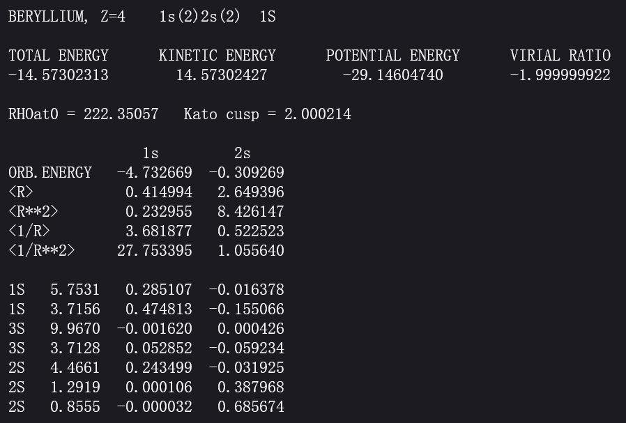
Atomic orbitals calculated by the Hartree-Fock-Roothaan method have been recalculated by Carlos Bunge and others and are available on-line at http://www.ccl.net/cca/data/atomic-RHF-wavefunctions/tables.

（ 该链接仍可用，你可以戳[这里]打开网站。 ）

Here is a screen shot of the results for Be atom from the website http://www.ccl.net/cca/data/atomic-RHF-wavefunctions/tables, so we can know the orbitals of a beryllium atom. For instance we can have $\psi_{2s}$:

$\psi_{2s} = -0.016378 S_{1s}(\zeta=5.7531) - 0.155066S_{1s}(\zeta=3.7156) \\[3mm] +0.000426S_{3s}(\zeta=9.9670) - 0.059234S_{3s}(\zeta=3.7128) \\[3mm] -0.031925S_{2s}(\zeta=4.4661) + 0.387968S_{2s}(\zeta=1.2919) + 0.685674S_{2s}(\zeta=0.8555)$

9.8 Correlation Energy Is the Difference Between the Hartree-Fock Energy and the Exact Energy

In Section 9.3, we defined a correlation energy ($E_{corr}$) by the equation

$E_{corr} = E_{exact} - E_{HF}$

Altough the Hartree-Fock energy for a helium atom is almost 99% of the exact energy, the difference is of the order of the strength of a chemical bond. The correlation energy increases with the number of electrons, so the inclusion of correlation is an important goal in quantum chemistry.

There is a method that is based upon the Hartree-Fock approximation, but can be used to calculate energies much better than Hartree-Fock energies.

The ground state of a helium atom has the electron configuration $\psi_1(1)\psi_1(2)$. The orbital $\psi_2(r)$ is not occupied in the ground state, and is called a virtual orbital.

We can form an excited state by promoting an electron from the ground-state orbital $\psi_1$ to the virtual orbital $\psi_2$. For example, $\psi_2(1)\psi_2(2)$ represents an electron configuration where both electrons are in the orbital $\psi_2$. Instead of using just $\psi_1(1)\psi_1(2)$, we could use

$\Psi_{CI}(1,2) = c_1\psi_1(1)\psi_1(2) + c_2\psi_2(1)\psi_2(2)$

this leads to the secular equation

$\left| \begin{matrix} H_{11}-E &H_{12} \\ H_{12} &H_{22}-E \end{matrix} \right| =0$

where

H_{11} = \bra {\psi_1(1)\psi_1(2)} \hat H \ket {\psi_1(1)\psi_1(2)} \\[3mm] H_{12} = \bra {\psi_1(1)\psi_1(2)} \hat H \ket {\psi_2(1)\psi_2(2)} \\[3mm] H_{22} = \bra {\psi_2(1)\psi_2(2)} \hat H \ket {\psi_2(1)\psi_2(2)}

Calculating in this way, we obtain $E=-2.87541E_h$ as the lower root. The difference between this value and the Hartree-Fock energy is $\Delta E=-0.01374E_h$, which is about one-third of the correlation energy. We also obtain the $\Psi_{CI}(1,2)$

$\Psi_{CI}(1,2) = 0.998864\psi_1(1)\psi_1(2) - 0.047644\psi_2(1)\psi_2(2)$

showing that $\psi_1(1)\psi_2(2)$ is the dominant contribution.

An advantage of this procedure is that all the necessary integrals had already been calculated in the previous Hartree-Fock calculation. A much more important feature, however, is that it becomes essentially exact in the limit.

If we use a Hartree-Fock orbital that is a linear combination of K Slater orbitals, instead of just two. The first orbital (the one of lowest energy) is doubly occupied in the ground state of a helium atom, and the remaining K - 1 orbitals are virtual orbitals. We can use all these orbitals to form many-electron configurations and write $\Psi_{CI}(1,2)$ as

$\Psi_{CI}(1,2) = \sum_i \sum_j c_{ij} \psi_i(1)\psi_j(2)$

The method we are describing is called configuration interaction(CI). As we use larger and larger basis sets and include more and more configurations, we approach the exact result.

（ 组态相互作用方法作为一种经典的后Hartree-Fock方法可以更好的接近HF极限，同时在理解层面上也与化学直觉相符。 ）

9.9 A Term Symbol Gives a Detailed Description of an Electron Configuration

In this section, we shall discuss term symbols for multielectron atoms.

The scheme we will present here is based upon the idea of determining the total orbital angular momentum $L$ and the total spin angular momentum $S$ and then adding $L$ and $S$ together vectorially to obtain the total angular momentum $J$. The result of such a calculation, called Russell-Saunders coupling, is presented as an atomic term symbol, which has the form

$^{2S+1}L_J$

In a term symbol, $L$ is the orbital angular-momentum quantum number, $S$ is the spin quantum number, and $J$ is the angular-momentum quantum number. We will see that $L$ will necessarily have values such as 0,1,2,… Similar to assigning the letters s,p,d, and f to the values l=0,1,2, and 3 of the orbital angular momentum for the hydrogen atom, we will make the following correspondence:

$\begin{matrix} L=&0\ &1\ &2\ &3\ &4\ &5 &\cdots \\ &S\ &P\ &D\ &F\ &G\ &H\ &\cdots \end{matrix}$

We will also see that the spin quantum nwnber S will necessarily have values such as $0, \frac 12, 1, \frac 32,\cdots$ , and so the $2S+1$ left superscript on a term symbol will have values such as 1, 2, 3, … The quantity $2S+1$ is called the spin multiplicity. Thus, ignoring for now the subscript $J$, term symbols will be of the type

$^3S \quad {}^2D \quad {}^1P$

The orbital angular momentun and the spin angular momentum are given by the vector sums

$\bold L = \sum_i \bold I_i$

$\bold S = \sum_i \bold s_i$

The z components of $\bold L$ and $\bold S$ are given by the scalar sums

$L_z = \sum_i l_{zi} = \sum_i m_{li} = M_L$

$S_z = \sum_i s_{zi} = \sum_i m_{si} = M_S$

Just as the z component of $\bold l$ can assume the $2l+1$ values $m_l=l,l-1,\cdots,0,\cdots,-l+1,-l$, the z component of $\bold L$ can assume the $2L+1$ values $M_L=L,L-1,\cdots,0,\cdots,-L+1,-L$.

Similarly, $M_S$ can take on the $2S+1$ values $S,S-1,\cdots,0,\cdots,-S+1,-S$. Thus, the spin multiplicity is simply the $2S+1$ projections that the z component of $\bold S$ can assume.

Let’s consider the electron configuration $ns^2$.

$\begin{matrix} m_{l1} &m_{s1} &m_{l2} &m_{s2} \quad &M_L &M_S \\[3mm] 0 &+\frac 12 &0 &-\frac 12 \quad &0 &0 \end{matrix}$

The total angular momentum $J$ is given by $\bold J = \bold L + \bold S$. And the only value of its z component is

$J_z = L_z + S_z = (M_L + M_S) = M_J =0$

which implies that $J=0$. So we find that the term symbol corresponding to an $ns^2$ electron configuration is $^1S_0$ (singlet S zero).

Notice that $M_L$ and $M_S$ are necessarily equal to zero for completely filled subshells because for every electron with a negative value of $m_{li}$, there is another electron with a corresponding positive value to cancel it; the same holds true for the values of $m_{Si}$. Thus, we can ignore the electrons in completely filled subshells when considering other electron configurations.

Another example of an electron configuration is $1s^12s^1$. The possible sets of values of $m_{l1}$, $m_{s1}$, $m_{l2}$ and $m_{s2}$ that are consistent with each value of $M_L$ and $M_S$ are called microstates. There are four microstates in this example:

$\begin{matrix} m_{l1} &m_{s1} &m_{l2} &m_{s2} \quad &M_L &M_S \\[3mm] 0 &+\frac 12 &0 &+\frac 12 \quad &0 &1 \\[3mm] 0 &+\frac 12 &0 &-\frac 12 \quad &0 &0 \\[3mm] 0 &-\frac 12 &0 &+\frac 12 \quad &0 &0 \\[3mm] 0 &-\frac 12 &0 &-\frac 12 \quad &0 &-1 \\[3mm] \end{matrix}$

We can obtain two pairs of $L=0,S=1$ and $L=0,S=0$, along with their possible values of $M_J$, can be summarized as

$\begin{aligned} &L=0,S=1 &&L=0,S=0 \\ &M_L=0,M_S=1,0,-1 &&M_L=0,M_S=0 \\ &M_J=M_L+M_S=1,0,-1 &&M_J=M_L+M_S=0 \end{aligned}$

The two term symbols corresponding to the electron configuration $1s^12s^1$ are

$^3S_1 \quad and \quad {}^1S_0$

The $^3S_1$ is called a triplet S state. We will see below that the triplet state ($^3S_1$) has a lower energy than the singlet state ($^1S_0$).

9.10 The Allowed Values of $J$ Are $L+S, L+S-1,\cdots, |L-S|$

We will consider a carbon atom, whose ground-state electron configuration is $1s^22s^22p^2$. We have shown previously that we do not need to consider completely filled subshells. Consequently, we can focus on the electron configuration $2p^2$.

We are going to assign two electrons to two of six possible spin orbitals, $(m_l,m_s)=(1,1/2),(1,-1/2),(0,1/2),(0,-1/2),(-1,1/2),(-1,-1/2)$. There are six choices for the first spin orbital and five choices for the second. Because the electrons are indistinguishable, however, the order of the two spin orbitals chosen is irrelevant. Thus, we should divide the 30 choices by 2 to give 15 as the number of distinct ways of assigning the two electrons to the six spin orbitals.

Generally, the number of distinct ways to assign N electrons to G spin orbitals belonging to the same subshell (equivalent orbitals) is given by

$\frac {G!}{N!(G-N)!}$

To determine the 15 possible sets of $m_{l1},m_{s1},m_{l2},m_{s2}$ for an $np^2$ electron configuration, we first determine the possible values of $M_L$ and $M_S$.

Because $m_{11}$ and $m_{12}$ can both have a maximum value of 1, the maximum value of $M_L$ is 2, and so its possible values are 2, 1, 0, -1, and -2. Similarly, $M_S$'s possible values are 1,0,-1.

So we can deduce the partially specified term symbols, $^1D$, $^3P$, and $^1S$. To complete the specification of these term symbols, we must determine the possible values of $J$ in each case.

Recall that $M_J=M_L+M_S$, and we can implies $J$. In summary, the electronic states associated with an $np^2$ configuration are

$^1D_2,\ ^3P_0,\ ^3P_1,\ ^3P_2,\ ^1S_0$

The degeneracies of these states are 5,1,3,5,1, or $2J+1$, which adds up to 15.

The values of $J$ for the term symbol can be determined in terms of the values of $L$ and $S$ if we recall that

$\bold J = \bold L + \bold S$

The largest value that $J$ can have is in the case when both $\bold L$ and $\bold S$ are pointing in the same direction, so that $J=L+S$. The smallest value that $J$ can have is when $\bold L$ and $\bold S$ are pointing in opposite directions, so that $J=|L-S|$.

$J=L+S,\ L+S-1,\ L+S-2,\ \cdots,\ |L-S|$

There is a useful consistency test between microstates and $(2S+1)(2L+1)$. Applying this result to the $np^2$ case gives

$(^1S)(1\times 1)+(^3P)(3\times 3)+(^1D)(1\times 5)=15$

9.11 Hund’s Rules Are Used to Determine the Term Symbol of the Ground Electronic State

Although we could calculate the energy associated with each state, in practice, the various states are ordered according to three empirical rules formulated by the German spectroscopist Friedrich Hund. Hund’s rules are as follows:

1. The state with the largest value of $S$ is the most stable (has the lowest energy), and stability decreases with decreasing $S$.
2. For states with the same value of $S$, the state with the largest value of $L$ is the most stable.
3. If the states have the same value of $L$ and $S$, then for a subshell that is less than half-filled, the state with the smallest value of $J$ is the most stable; for a subshell that is more than half-filled, the state with the largest value of $J$ is the most stable.

（ Hund规则优先考虑$S$，其次是$L$，最后是$J$。实际上是我们在无机化学中学过的Hund规则的完整版。通过应用Hund第一到第三规则，可以确定能量最低，即最稳定的微观状态。 ）

9.12 Atomic Term symbols Are Used to Describe Atomic Spectra

Atomic term symbols are sometimes called spectroscopic term symbols because atomic spectral lines can be assigned to transitions between states that are described by atomic term symbols.

The energies of the electronic states of many atoms and ions are available online at a website https://www.nist.gov/pml/atomic-spectra-database maintained by the National Institute of Standards and Technology (NIST).

（ 原书中提供的链接为旧版本链接，我在上文中已修改为新版本链接，你可以戳[这里]访问，网站提供了光谱线、原子基态能量和电离能等数据。 ）

The spectrum of atomic sodium is due to transitions from one state to another. As for many of the systems that wwe have studied earlier, not all transitions are allowed; there are selection rules that govern which transitions are allowed.

For Russell-Saunders coupling, the selection rules for multielectron atoms are

$\begin{aligned} \Delta L &= 0, \pm 1 \quad (L=0 \nrightarrow L=0) \\ \Delta S &= 0 \\ \Delta J &= 0, \pm 1 \quad (J=0 \nrightarrow J=0) \end{aligned}$

The selection rules tell us that $^2P \rightarrow {}^2S$ transitions are allowed, but $^2D \rightarrow {}^2S$ are not allowed because $\Delta L=2$. Furthermore, $^2S \rightarrow {}^2S$ transitions are not allowed because $L=0$ in both states.

We should point out that the selection rules presented here are useful only for small spin-orbit coupling, and so they apply only to atoms with small atomic numbers. As the atomic number increases, the selection rules break down.

9.13 Russell-Saunders Coupling Is Most Useful for Light Atoms

In addition to the usual kinetic energy and electrostatic terms in the Hamiltonian operator of a many-electron atom, there are a number of magnetic and spin terms. The most important of these magnetic and spin terms is the spin-orbit interaction term.

$\hat H = -\frac 12 \sum_j \nabla_j^2 - \sum_j \frac {Z}{r_j} + \sum_{i<j} \frac 1{r_{ij}} + \sum_j\zeta(r_j)\bold I_j \cdot \bold s_j$

where $\bold I_j$ and $\bold s_j$ are the individual electronic orbital momenta and spin angular momenta, respectively, and where $\zeta(r_j)$ is a scalar function of $r_j$ whose form is not necessary here.

We can abbreviate the equation by writing

$\hat H = \hat H_0 + \hat H_{ee} + \hat H_{so}$

where $\hat H_0$ represents the first two terms (no interelectronic interactions), $\hat H_{ee}$ represents the third term (interelectronic repulsion), and $\hat H_{so}$ represents the fourth term (spin-orbit coupling).

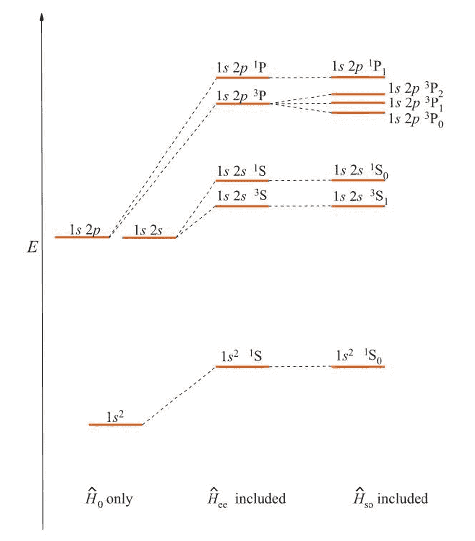
Figure 9.2 is a schematic diagram of howw the energies of the $1s^2$, $1s2s$, and $1s2p$ electron configurations of a helium atom are split by the $\hat H_{ee}$ term and then by the $\hat H_{so}$ term.

Note that the energies in this figure are not to scale, the splitting due to spin-orbit coupling is much smaller than that due to electron-electron repulsion. The scheme is known as Russell-Saunders coupling,
and is usually a very good approximation for light atoms.

As the atomic number of the atom increases, the spin-orbit term becomes larger than the interelectronic term, and now $H_{ee}$ can be considered to be a small perturbation relative to the other terms in $H$. In this case $L$ and $S$ are no longer meaningful, and individual total angular momenta $\bold j_i=\bold I_i + \bold s_i$ become the approximately conserved quantities.

（ Russell-Saunders耦合，或称L-S耦合往往对于轻原子比较有效，对于重原子则往往使用j-j耦合。 ）

总结

本章开始涉及多电子原子体系，相较氢原子更加复杂，因此需要各种方法求得近似解，并确保近似解有足够的精度。介绍了Hartree-Fock方法和后H-F方法，以及光谱项的相关内容。