《Quantum Chemistry》章末总结8

第八章是解薛定谔方程的近似方法，介绍变分法和微扰法。

Chapter 8 Approximation Methods

8.1 The Variational Method Provides an Upper Bound to the Ground-State Energy of a System

We will first illustrate the variational method. Consider the ground state of some arbitrary system. The ground-state wave function $\psi_0$ and energy $E_0$ satisfy the Schrödinger equation:

$\hat H \psi_0 = E_0\psi_0$

We can obtain:

$E_0=\frac {\langle \psi_0|\hat H|\psi_0 \rangle}{\langle \psi_0|\psi_0 \rangle}$

A beautiful theorem says that if we substitute any other function $\phi$ for $\psi_0$ into the equation and calculate the corresponding energy:

$E_{\phi}=\frac {\langle \phi|\hat H|\phi \rangle}{\langle \phi|\phi \rangle}$

then $E_{\phi}$ will be greater than the ground-state energy $E_0$. In an equation, we have the variational principle:

$E_{\phi} \ge E_0$

where the equality holds only if $\phi=\psi_0$, the exact wave function.

The variational principle says that we can calculate an upper bound to $E_0$ by using any trial function we wish. The closer $\phi$ is to $\psi_0$ in some sense, the closer $E_{\phi}$ will be to $E_0$.

We can choose a trial function $\phi$ such that it depends upon some arbitrary
parameters, $\alpha,\beta,\gamma,\cdots$, called variational parameters. The energy also will depend upon these variational parameters:

$E_{\phi}(\alpha,\beta,\gamma,\cdots) \ge E_0$

Now we can minimize $E_{\phi}$ with respect to each of the variational parameters and thus approach the exact ground-state energy $E_0$.

（ 变分法依赖于变分原理，即试验函数的能量一定大于等于基态能量。那么对于任意给定的试验函数，总有办法令其尽可能小，尽可能接近$\psi_0$，则能量就会更接近$E_0$。 ）

As a example, we will use the variational method to estimate the ground-state energy of a helium atom:

$\hat H=-\frac {\hbar^2}{2m_e}(\nabla^2_1+\nabla^2_2)-\frac {2e^2}{4\pi \epsilon_0} \left(\frac 1{r_1}+\frac 1{r_2} \right)+\frac {e^2}{4\pi \epsilon_0}\frac 1{r_{12}}$

The Schrödinger equation cannot be solved exactly for this system because of the term involving $r_{12}$.

We can rewrite the equation and obtain:

$\hat H=\hat H_H(1)+\hat H_H(2)+\frac {e^2}{4\pi \epsilon_0}\frac 1{r_{12}}$

where:

$\hat H_H(j)=-\frac {\hbar^2}{2m_e}\nabla_j^2-\frac {2e^2}{4\pi\epsilon_0}\frac 1{r_j} \quad j=1\ and\ 2$

is the Hamiltonian operator for a single electron around a helium nucleus. If we ignore the interelectronic repulsion term, then the Hamiltonian operator is separable and the ground-state wave function would be:

$\phi_0(\boldsymbol r_1,\boldsymbol r_2)=\psi_{1s}(\boldsymbol r_1)\psi_{1s}(\boldsymbol r_2)$

where:

$\psi_{1s}(\boldsymbol r_j)=\left(\frac {Z^3}{\pi a_0} \right)^{1/2} e^{-Zr_j/a_0} \quad j=1\ or\ 2$

where $a_0=4\pi\epsilon_0\hbar^2/m_ee^2$. We use these equation as a trial function using $Z$ as a variational constant. Thus, we must evaluate:

$E(Z)=\int \phi_0(\boldsymbol r_1,\boldsymbol r_2)\hat H \phi_0(\boldsymbol r_1,\boldsymbol r_2)d\boldsymbol r_1 d\boldsymbol r_2$

The integral is a bit lengthy, we can get the results:

$E(Z)=\frac {m_ee^4}{16\pi^2\epsilon_0^2\hbar^2}\left(Z^2-\frac {27}{8}Z \right)$

It is convenient to express $E$ in units of $m_ee^4/16\pi^2\epsilon_0^2\hbar^2$. If we minimize $E(Z)$ with respect to $Z$, we find that $Z_{min}=27/16$. So we get:

$E_{min}=-\left(\frac {27}{16} \right)^2=-2.8477$

which is in good agreement with the experimental result of $-2.9033$. Thus, we achieve a fairly good result, considering the simplicity of the trial function.

（ 在氦原子能量的近似计算中，我们选择的试验函数为$\phi=\psi(\boldsymbol r_1)\psi(\boldsymbol r_2)$，试验函数表示为电子波函数的乘积，说明哈密顿算符是可分离的，即忽略了电子间的相互作用的近似，不过结果准确度还是足够令人满意的。 ）

8.2 A Trial Function That Depends Linearly on the Variational Parameters Leads to a Secular Determinant

As another example of the variational method, consider a particle in a one-dimensional box. we should expect it to be symmetric about $x=a/2$ and to go to zero at the walls. One of the simplest functions with these properties is $x^n(a-x)^n$, where $n$ is an integer. Consequently, let’s estimate $E_0$ by using:

$\phi=c_1x(a-x)+c_2x^2(a-x)^2$

as a trial function, where $c_1$ and $c_2$ are to be determined variationally—that is, where $c_1$ and $c_2$ are the variational parameters. With this trial function, we can get the result:

$E_{min}=0.125\,002\frac {h^2}{ma^2}$

compared with:

$E_{exact}=0.125\,000\frac {h^2}{ma^2}$

So we see that using a trial function with more than one parameter can produce impressive results. The price we pay is a correspondingly more lengthy calculation.

Fortunately, there is a systematic way to handle a trial function, which can be written generally as:

$\phi=\sum^N_{n=1}c_nf_n$

Consider:

$\phi = c_1f_1+c_2f_2$

Then:

$\begin{aligned}\int \phi\hat H\phi d\tau &= \int(c_1f_1+c_2f_2)\hat H(c_1f_1+c_2f_2) d\tau \\[3mm] &= c_1^2H_{11}+c_1c_2H_{12}+c_1c_2H_{21}+c_2^2H_{22} \end{aligned}$

where the $H_{ij}$ are given by:

$H_{ij}=\int f_i\hat H f_j d\tau = \langle i|\hat H|j \rangle$

Becasue $\hat H$ is Hermitian, the $H_{ij}$ are symmetric; in other words, $H_{ij}=H_{ji}$. So:

$\int \phi\hat H\phi d\tau = c_1^2H_{11} + 2c_1c_2H_{12} + c_2^2H_{22}$

Similarly, we have:

$\int \phi^2 d\tau = c_1^2S_{11} + 2c_1c_2S_{12} + c_2^2S_{22}$

where:

$S_{ij}=S_{ji}=\int f_if_j d\tau = \langle i|j \rangle$

The quantities $H_{ij}$ and $S_{ij}$ are called matrix elements. We can calculate the corresponding energy with the expression of matrix elements:

$E(c_1,c_2)=\frac {c_1^2H_{11} + 2c_1c_2H_{12} + c_2^2H_{22}}{c_1^2S_{11} + 2c_1c_2S_{12} + c_2^2S_{22}}$

$E$ is a function of the variational parameters $c_1$ and $c_2$, we differentiating $E(c_1,c_2)$ with respect to $c_1$. We find that:

$(2c_1S_{11}+2c_2S_{12})E + \frac {\partial E}{\partial c_1} (c_1^2S_{11}+2c_1c_2S_{12}+c_2^2S_{22}) = 2c_1H_{11}+2c_2H_{12}$

Because we are minimizing $E$ with respect to $c_1$, $\partial E / \partial c_1=0$, so the equation becomes:

$c_1(H_{11}-ES_{11}) + c_2(H_{12}-ES_{12})=0$

Similarly, differentiating $E$ with respect to $c_2$:

$c_1(H_{12}-ES_{12}) + c_2(H_{22}-ES_{22})=0$

There is a nontrivial solution, if and only if the determinant of the coefficients vanishes:

$\left|\begin{matrix} H_{11}-ES_{11}& H_{12}-ES_{12} \\ H_{12}-ES_{12}& H_{22}-ES_{22} \end{matrix}\right| =0$

Thus, we obtain a secular determinant and a secular equation.

The quadratic secular equation gives two values for $E$, and we take the smaller of the two as our variational approximation for the ground-state energy.

（ 将选取的试验函数计算出的能量用矩阵元表示，那么最小能量的计算就转化为了久期方程的计算，这是变分法的一种通用计算套路。 ）

Let’s go back to solving the problem of a particle in a one-dimensional box. For convenience, we will set $a=1$. In this case:

$f_1=x(1-x) \quad and \quad f_2=x^2(1-x)^2$

and the matrix elements are:

$H_{11}=\frac {\hbar^2}{6m} \quad S_{11}=\frac {1}{30} \\[3mm] H_{12}=H_{21}=\frac {\hbar^2}{30m} \quad S_{12}=S_{21}=\frac {1}{140} \\[3mm] H_{22}=\frac {\hbar^2}{105m} \quad S_{22}=\frac {1}{630}$

The secular determinant gives:

$\left |\begin{matrix}\frac 16 - \frac {\epsilon}{30}& \frac 1{30} - \frac {\epsilon}{140} \\[3mm] \frac 1{30} - \frac {\epsilon}{140}& \frac 1{105} - \frac {\epsilon}{630} \end{matrix}\right | =0$

where $\epsilon=Em/\hbar^2$. The roots of secular equation is:

$\epsilon = \frac {56\pm \sqrt{2128}}{2} = 51.065 \quad and \quad 4.93487$

We choose the smaller root and obtain:

$E_{min}=4.93487\frac {\hbar^2}{m} = 0.125\,002\frac {h^2}{m}$

The excellent agreement here (remember $E_{exact}=0.125\,000\frac {h^2}{m}$) is better than should be expected normally for such a simple trial function.

We can also determine the normalized trial function for our variational treatment of a particle in a box:

$\frac {c_2}{c_1}= -\frac {H_{11}-ES_{11}}{H_{12}-ES_{12}} = 1.13342$

$\phi(x)=c_1[x(1-x)+1.13342x^2(1-x)^2]$

$\int_0^1\phi^2(x)dx = c_1^2 \int_0^1 [x(1-x)+1.13342x^2(1-x)^2]^2 dx =1$

So we can obtain:

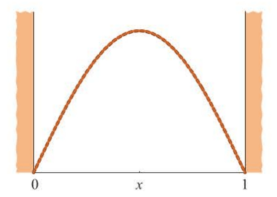
$\phi(x)=4.40378x(1-x) + 4.99133x^2(1-x)^2$

Figure 8.1 is a comparison of the optimized and normalized trial function with the exact ground-state particle-in-a-box wave function, $\psi_1(x)=\sqrt 2 \sin\pi x$. The two curves are essentially the same.

If we use a linear combination of $N$ functions, instead of using a linear combination of two functions as we have done so far, then we obtain $N$ simultaneous linear algebraic equations for the $c_j$'s. We can express compactly by using the matrix notation:

$\mathbf H c = E\mathbf S c$

where $\mathbf H$ is an $N\times N$ matrix with matrix elements $H_{ij}$, $\mathbf S$ is an $N\times N$ matrix with matrix elements $S_{ij}$, and $c$ is an $N\times 1$ column matrix whose elements are $c_j$.

To have a nontrivial solution to this set of homogeneous equations, we must have:

$|\mathbf H -E\mathbf S|=0$

The determination of the smallest root must usually be done numerically for values of $N$ larger than two. This is actually a standard numerical problem, and a number of packaged computer programs do this.

（ 当试验函数的选取更加精细，它可以表示为N个函数的线性组合，那么我们就会得到一个N阶久期行列式和N阶久期方程，同样是把它解出来并选择能量的最小值，然后就可以解出相应的试验函数。 ）

8.3 Trial Functions Can Be Linear Combinations of Functions That Also Contain Variational Parameters

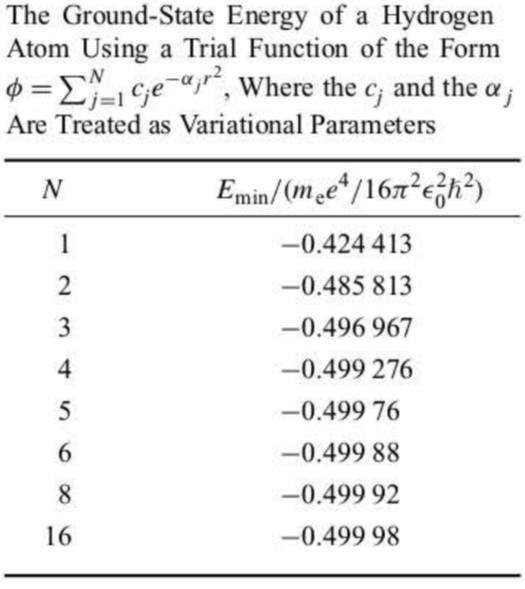
An example of a trial function for the hydrogen atom is:

$\phi = \sum_{j=1}^N c_je^{-\alpha_j r^2}$

where the $c_j$'s and the $\alpha_j$'s are treated as variational parameters. $\phi$ is linear only in the $c_j$ but not in the $\alpha_j$. The minimization of $E$ with respect to the $c_j$ and $\alpha_j$ is fairly complicated, involving $2N$ parameters, and must be done numerically.

（ 试验函数可以是一系列函数的线性组合，同时每一个函数都可以另外包含一个参数。当N逐渐增大，准确度也逐渐提高，但是计算的复杂度也会提高，如何从中做出适当的取舍是另一个重要的问题。 ）

8.4 Perturbation Theory Expresses the Solution to One Problem in Terms of Another Problem That Has Been Solved Previously

Suppose we wish to solve the Schrödinger equation for some particular system, but we are unable to find an exact solution as we have done for a harmonic oscillator, a rigid rotator, and a hydrogen atom in previous chapters. It turns out that most systems cannot be solved exactly; some specific examples are a helium atom, an anharmonic oscillator, and a nonrigid rotator.

For example, the Hamiltonain operator for a helium atom is:

$\hat H=-\frac {\hbar^2}{2m_e}(\nabla^2_1+\nabla^2_2)-\frac {2e^2}{4\pi \epsilon_0} \left(\frac 1{r_1}+\frac 1{r_2} \right)+\frac {e^2}{4\pi \epsilon_0}\frac 1{r_{12}}$

and it can be written in the form:

$\hat H=\hat H_H(1)+\hat H_H(2)+\frac {e^2}{4\pi \epsilon_0}\frac 1{r_{12}}$

where:

$\hat H_H(j)=-\frac {\hbar^2}{2m_e}\nabla_j^2-\frac {2e^2}{4\pi\epsilon_0}\frac 1{r_j} \quad j=1\ and\ 2$

Another example of a problem that could be solved readily if it were not for additional terms in the Hamiltonian operator is an anharmonic oscillator.

$\hat H=-\frac {\hbar^2}{2\mu}\frac {d^2}{dx^2} + \frac 12kx^2 + \frac 16\gamma_3x^3 + \frac 1{24}\gamma_4x^4$

These two examples, with their Hamiltonian operators, introduce us to the basic idea behind perturbation theory.

In both of these cases, the total Hamiltonian operator consists of two parts, one for which the Schrödinger equation can be solved exactly and an additional term, whose presence prevents an exact solution. We call the first term the unperturbed Hamiltonian operator and the additional term
the perturbation.

We shall denote the unperturbed Hamiltonian operator by $\hat H^{(0)}$ and the perturbation by $\hat H^{(1)}$ and write:

$\hat H = \hat H^{(0)}+\hat H^{(1)}$

Associated with $\hat H^{(0)}$ is a Schrödinger equation, which we know how to solve, and so we have:

$\hat H^{(0)}\psi^{(0)} = E^{(0)}\psi^{(0)}$

where $\psi^{(0)}$ and $E^{(0)}$ are the known eigenfunctions and eigenvalues of $\hat H^{(0)}$.

（ 通俗地讲，微扰理论就是将复杂问题拆分，拆分为粗略的近似解+更精确的修正项。以氦原子为例，其哈密顿算符可以写成两个电子分别对核的作用（即$\hat H_H(1),\hat H_H(2)$）加上电子的相互作用（即$e^2/4\pi \epsilon_0 r_{12}$）。前者为非微扰项，可以精确地求解，后者则为微扰项，需要通过一些方法近似得到，而两部分加起来就是总的近似结果。 ）

8.5 Perturbation Theory Consists of a Set of Successive Corrections to an Unperturbed Problem

In this section, we shall derive the equation for a first-order correction to the energy.

In order to keep track of the order of our perturbation expansion, it is convenient to introduce a parameter $\lambda$ into the Hamiltonian operator:

$\hat H = \hat H^{(0)} + \lambda\hat H^{(1)}$

The factor $\lambda$ is simply a bookkeeping device that will help us identify to what order our resultant perturbation equations are valid. We shall see that terms linear in $\lambda$ give us what we call first-order corrections, terms in $\lambda^2$ give us second-order corrections, and so on.

It’s a fact that $\psi_n$ and $E_n$ will depend upon $\lambda$. We assume that we can express the $\psi_n$ and $E_n$ as power series in $\lambda$, so that:

$\psi_n = \psi_n^{(0)} + \lambda\psi_n^{(1)} + \lambda^2\psi_n^{(2)} + \cdots$

and:

$E_n = E_n^{(0)} + \lambda E_n^{(1)} + \lambda^2 E_n^{(2)} + \cdots$

We can obtain:

$(\hat H^{(0)} + \lambda\hat H^{(1)})(\psi_n^{(0)} + \lambda\psi_n^{(1)} + \lambda^2\psi_n^{(2)} + \cdots) = (E_n^{(0)} + \lambda E_n^{(1)} + \lambda^2 E_n^{(2)} + \cdots)\times(\psi_n^{(0)} + \lambda\psi_n^{(1)} + \lambda^2\psi_n^{(2)} + \cdots)$

Each side of this equation is an expresion in $\lambda$, which can be written as:

$\begin{aligned} &(\hat H^{(0)}\psi_n^{(0)} - E_n^{(0)}\psi_n^{(0)})+(\hat H^{(0)}\psi_n^{(1)}+\hat H^{(1)}\psi_n^{(0)}-E_n^{(0)}\psi_n^{(1)}-E_n^{(1)}\psi_n^{(0)})\lambda \\[3mm] &+ (\hat H^{(0)}\psi_n^{(2)}+\hat H^{(1)}\psi_n^{(1)}-E_n^{(0)}\psi_n^{(2)}-E_n^{(1)}\psi_n^{(1)}-E_n^{(2)}\psi_n^{(0)})\lambda^2 + O(\lambda^3)=0 \end{aligned}$

where $O(\lambda^3)$ means terms of order $\lambda^3$ and higher. Notice that both terms in the first set of parentheses, the coefficient of $\lambda^0$, are of zero order; all four terms in the second set of parentheses, the coefficient of $\lambda^1$, are of first order; and so on.

Because $\lambda$ is an arbitrary parameter, the coefficients of each power of $\lambda$ must equal zero separately. The terms in the first set of parentheses equal zero. Let’s look at the coefficent of $\lambda^1$:

$\hat H^{(0)}\psi_n^{(1)}+\hat H^{(1)}\psi_n^{(0)}=E_n^{(0)}\psi_n^{(1)}+E_n^{(1)}\psi_n^{(0)}$

The equation can be simplified considerably by multiplying both sides from the left by $\psi_n^{(0)*}$ and integrating over all space:

$\langle \psi_n^{(0)}|\hat H^{(0)}-E_n^{(0)}|\psi_n^{(1)} \rangle + \langle \psi_n^{(0)}|\hat H^{(1)}|\psi_n^{(0)} \rangle = E_n^{(1)}\langle \psi_n^{(0)}|\psi_n^{(0)} \rangle$

The first term on the left side is equal to zero, because $\hat H^{(0)}-E^{(0)}$ is Hermitian, and so we get:

$E_n^{(1)} = \langle \psi_n^{(0)}|\hat H^{(1)}|\psi_n^{(0)} \rangle$

Equation gives $E_n^{(1)}$, the first-order correction to $E_n^{(0)}$. Then, the energy is given by:

$E_n=E_n^{(0)} + E_n^{(1)} = E_n^{(0)} + \langle \psi_n^{(0)}|\hat H^{(1)}|\psi_n^{(0)} \rangle \quad (first\ order)$

We can apply perturbation theory to a helium atom. For simplicity, we will consider only the ground-state energy. If we consider the interelectronic repulsion term, $e^2/4\pi\epsilon_0r_{12}$, to be the perturbation, then the unperturbed wave functions and energies are the hydrogen-like quantities given by:

$\begin{aligned} &\hat H^{(0)}=\hat H_H(1) + \hat H_H(2) \\[3mm] &\psi^{(0)}=\psi_{1s}(r_1,\theta_1,\phi_1) \psi_{1s}(r_2,\theta_2,\phi_2) \\[3mm] &E^{(0)} = -\frac {Z^2m_ee^4}{32\pi^2\epsilon_0^2\hbar^2n_1^2}- \frac {Z^2m_ee^4}{32\pi^2\epsilon_0^2\hbar^2n_2^2} \end{aligned}$

and:

$\hat H^{(1)} = \frac {e^2}{4\pi\epsilon_0r_{12}}$

With $Z=2$, we have:

$E^{(1)} = \int\int d\boldsymbol r_1 d\boldsymbol r_2 \psi_{1s}(\boldsymbol r_1)\psi_{1s}(\boldsymbol r_2) \frac {e^2}{4\pi\epsilon_0r_{12}}\psi_{1s}(\boldsymbol r_1)\psi_{1s}(\boldsymbol r_2)$

This integral is a little lengthy, the final result is:

$E^{(1)}= \frac {5Z}{8} \left(\frac {m_ee^4}{16\pi^2\epsilon_0^2\hbar^2} \right)$

In units of $m_ee^4/16\pi^2\epsilon_0^2\hbar^2$, we have:

$E=E^{(0)}+E^{(1)}=-Z^2 + \frac 58Z$

Letting $Z=2$ gives $-2.750$ compared with our simple variational result ($-2.8477$) and the experiment result of $-2.9033$. So we see that first-order perturbation theory gives a result that is about 5% in error.

It turns out that second-order perturbation theory gives $-2.910$ and that higher orders give $-2.9037$. Thus, we see that both the variational method and the perturbation theory are able to achieve very good results if carried far enough.

8.6 Selection Rules Are Derived from Time-Dependent Perturbation theory

The spectroscopic selection rules determine which transitions from one state to another are possible. The very nature of transitions implies a time-dependent phenomenon, so we must use the time-dependent Schrödinger equation:

$\hat H \Psi = i\hbar \frac {\partial \Psi}{\partial t}$

and $\psi_n(\boldsymbol r)$ satisfies the time-independent Schrödinger equation:

$\hat H \psi_n(\boldsymbol r) = E_n \psi_n(\boldsymbol r)$

Consider now a molecule interacting with electromagnetic radiation. The electromagnetic field may be written approximately as:

$\boldsymbol E = \boldsymbol E_0 \cos 2\pi\nu t$

If $\boldsymbol \mu$ is the dipole moment of the molecule, then the Hamiltonian operator for the interaction of the electric field with the molecule is:

$\hat H^{(1)} = -\boldsymbol \mu \cdot \boldsymbol E = -\boldsymbol \mu \cdot \boldsymbol E_0 \cos 2\pi\nu t$

So the $\hat H$ is:

$\hat H = \hat H^{(0)} + \hat H^{(1)} = \hat H^{(0)} - \boldsymbol \mu \cdot \boldsymbol E_0 \cos 2\pi\nu t$

We will se below that the time-dependent term $\hat H^{(1)}$ can cause transitions from one stationary state to another.

To solve the equation, we will treat the time-dependent term $\hat H^{(1)}$ as a small perturbation. The procedure we will use is called time-dependent perturbation theory.

For simplicity of notation we will consider only a two-state system.

$\Psi_1(t) = \psi_1 e^{-iE_1t/\hbar} \quad and \quad \Psi_2(t) = \psi_2 e^{-iE_2t/\hbar}$

Assume now that initially the system is in state 1. We let the perturbation begin at $t=0$ and assume that $\Psi(t)$ is a linear combination of $\Psi_1(t)$ and $\Psi_2(t)$ with coefficients that depend upon time:

$\Psi(t) = a_1(t)\Psi_1(t) + a_2(t)\Psi_2(t)$

where $a_1(t)$ and $a_2(t)$ are to be determined.

We substitute the equation into the time-dependent Schrödinger equataion:

$\begin{aligned} &a_1(t)\hat H^{(0)}\Psi_1 + a_2(t)\hat H^{(0)}\Psi_2 + a_1(t)\hat H^{(1)}\Psi_1 + a_2(t)\hat H^{(1)}\Psi_2 \\[3mm] = &a_1(t)i\hbar \frac {\partial \Psi_1}{dt} + a_2(t)i\hbar \frac {\partial \Psi_2}{dt} + i\hbar\Psi_1 \frac {da_1}{dt} + i\hbar\Psi_2 \frac {da_2}{dt} \end{aligned}$

The first two terms on the both sides are the same, so we get:

$a_1(t)\hat H^{(1)}\Psi_1 + a_2(t)\hat H^{(1)}\Psi_2 = i\hbar\Psi_1\frac {da_1}{dt} + i\hbar\Psi_2\frac {da_2}{dt}$

We now multiply the equation by $\psi_2^*$ and integrate over the spatial coordinates to get:

$a_1(t)\int \psi_2^*\hat H^{(1)}\Psi_1 d\tau + a_2(t)\int \psi_2^*\hat H^{(1)}\Psi_2 d\tau \\[3mm] =i\hbar \frac {da_1}{dt} \int \psi_2^*\Psi_1 d\tau + i\hbar \frac {da_2}{dt} \int \psi_2^*\Psi_2 d\tau$

Solving the equation gives:

$i\hbar \frac {da_2}{dt} = a_1(t)e^{iE_2t/\hbar} \int \psi_2^* \hat H^{(1)} \Psi_1 d\tau + a_2(t)e^{iE_2t/\hbar} \int \psi_2^* \hat H^{(1)} \Psi_2 d\tau$

The system is initially in state 1, and so:

$a_1(0)=1 \quad and \quad a_2(0)=0$

Because $\hat H^{(1)}$ is considered a small perturbation, there are not enough transitions out of state 1 to cause $a_1$ and $a_2$ to differ appreciably from their initial values. Thus, as an approximation, we may replace $a_1(t)$ and $a_2(t)$ by
their initial values to get:

$i\hbar \frac {da_2}{dt} = \exp \left[\frac {-i(E_1-E_2)t}{\hbar} \right] \int \psi_2^*\hat H^{(1)}\psi_1 d\tau$

（ 微扰法的“微”字在此体现，由于扰动非常小，所以可以认为线性组合系数近似保持不变。 ）

For convenience only, we will take the electric field to be in the z direction, in which case we can write:

$\hat H^{(1)} = -\mu_zE_{0z} \cos\omega t = -\frac {\mu_z E_{0z}}{2}(e^{i\omega t} + e^{-i\omega t})$

$\frac {da_2}{dt} = -\frac {(\mu_z)_{12}E_{0z}}{2i\hbar} \left\{\exp \left[\frac {i(E_2-E_1+\hbar \omega)t}{\hbar} \right] + \exp \left[\frac {i(E_2-E_1-\hbar \omega)t}{\hbar} \right] \right\}$

Let’s integrate the equation between 0 and t to obtain:

$a_2(t) = \frac {(\mu_z)_{12}E_{0z}}{2} \left\{\frac {\exp [i(E_2-E_1+\hbar\omega)t/\hbar]-1}{E_2-E_1+\hbar\omega} + \frac {\exp [i(E_2-E_1-\hbar\omega)t/\hbar]-1}{E_2-E_1-\hbar\omega} \right\}$

Because we have taken $E_2 > E_1$, the so-called resonance denominators cause the second term in this equation to become much larger than the first term and to be of major importance in determining $a_2(t)$ when:

$E_2 - E_1 \approx \hbar \omega = h\nu$

Thus, we obtain in a natural way the Bohr frequency condition we have used repeatedly. When a system makes a transition from one state to another, it absorbs (or emits) a proton whose energy is equal to the difference in the energies of the two states.

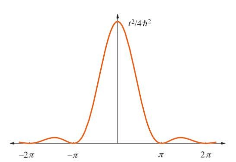
The probability of absorption or the intensity of absorption is proportional to the probability of observing the molecules to be in state 2, which is given by $a_2^*(t)a_2(t)$.

$P_{1\rightarrow 2}(\omega ,t) = a_2^*(t)a_2(t) = \frac {(\mu_z)^2_{12}E_{0z}^2 \sin^2 [(E_2-E_1-\hbar\omega)t/2\hbar]}{(E_2-E_1-\hbar\omega)^2}$

（ 上述的推导说明跃迁几率在能级能差等于$h\nu$时达到最大值，也即推出了波尔模型的频率条件。 ）

But that is not applicable under normal conditions because the irradiating source consists of at least a narrow band of frequencies, so the equation must be averaged over this band.

（ 一方面光源不是严格的单色光，另一方面分子解离发射荧光也会干扰吸收过程，这两点都会导致上式与实际情况产生偏差。 ）

If we let $g(\omega)$ be the frequency distribution of the irradiating source, then $P_{1\rightarrow 2}(\omega ,t)$ becomes:

$P_{1\rightarrow 2}(t) = (\mu_z)^2_{12} E_{0z}^2 \int_{band} \frac {\sin^2[(E_2-E_1-\hbar\omega)t/2\hbar]}{(E_2-E_1-\hbar\omega)^2} g(\omega)d\omega$

When $\omega = \omega_{12} = (E_2-E_1)/\hbar$, the $P_{1\rightarrow 2}(t)$ reaches its peak. So if $g(\omega)$ does not vary too strongly around $\omega_{12}$, then to a good approximation, we may take $g(\omega_{12})$ out from under the integral sign and write it as:

$P_{1\rightarrow 2}(t) = (\mu_z)^2_{12} E_{0z}^2 g(\omega_{12}) \int_{band} \frac {\sin^2[(E_2-E_1-\hbar\omega)t/2\hbar]}{(E_2-E_1-\hbar\omega)^2} d\omega$

Futhermore, because the integrand is peaked around $\omega=\omega_{12}$, we can write the integration limits as $-\infin$ to $\infin$ and write:

$P_{1\rightarrow 2}(t) = (\mu_z)^2_{12} E_{0z}^2 g(\omega_{12}) \int_{-\infin}^{\infin} \frac {\sin^2[(E_2-E_1-\hbar\omega)t/2\hbar]}{(E_2-E_1-\hbar\omega)^2} d\omega$

The result of the integration is:

$P_{1\rightarrow 2}(t) = \frac {\pi}{2} \left[\frac {(\mu_z)_{12}E_{0z}}{\hbar} \right]^2 tg(\omega_{12})$

The spectroscopic absorption coefficient is the rate at which transitions occur, and so equals the time derivative of $P_{1\rightarrow 2}$, or:

$W_{1\rightarrow 2} = \frac {\pi}{2} \left[\frac {(\mu_z)_{12}E_{0z}}{\hbar} \right]^2 g(\omega_{12})$

This formula simply says that there must be radiation at the frequency $\omega_{12}=(E_2-E_1)/\hbar$ for a transition to occur, which is just a formal statement of the Bohr frequency condition. The equation is a form of what is called Fermi’s golden rule.

总结

这一章从开学前开始写，过了一个月才写完，主要是开学后没有很多时间看了。

本章讨论了几种近似方法，包括变分法和微扰法，理解起来比前面的章节吃力不少。