《Quantum Chemistry》章末总结7

第七章是解氢原子，量子力学绕不开的关键部分。

Chapter 7 The Hydrogen Atom

7.1 The Schrödinger Equation for a Hydrogen Atom Can Be Solved Exactly

The electron and the proton in a hydrogen atom interact through a coulombic potential:

$V(r)=-\frac {e^2}{4\pi \epsilon_0r}$

where $e$ is the charge on the proton, $\epsilon_0$ is the permittivity of free space, and $r$ is the distance between the electron and the proton.

The Hamiltonian operator for a hydrogen atom is:

$\hat H=-\frac {\hbar^2}{2m_e}\nabla^2-\frac {e^2}{4\pi\epsilon_0r}$

where $m_e$ is the mass of the electron, and the Schrödinger equation is:

$-\frac {\hbar^2}{2m_e}\nabla^2\psi(r,\theta,\phi)+V(r)\psi(r,\theta,\phi)=E\psi(r,\theta,\phi)$

We substitute the Laplacian operator into the equation and write it as a more manageable form:

$-\hbar^2\frac {\partial}{\partial r} \left(r^2\frac {\partial\psi}{\partial r} \right)-\hbar^2 \left[\frac 1{\sin\theta} \left(\frac {\partial}{\partial \theta}\sin\theta\frac {\partial \psi}{\partial \theta}+\frac 1{\sin^2\theta}\frac {\partial^2\psi}{\partial \phi^2} \right) \right]+2m_er^2[V(r)-E]\psi(r,\theta,\phi)=0$

The second term here, the one containing all the $\theta$ and $\phi$ dependence, is nothing but $\hat L^2\psi$. Thus, we can write the Schrödinger equation in the form:

$-\hbar^2\frac {\partial}{\partial r} \left(r^2\frac {\partial\psi}{\partial r} \right)+\hat L^2\psi+2m_er^2[V(r)-E]\psi(r,\theta,\phi)=0$

Notice now that the entire left side of the equation consists of a part that depends upon only $r$ and a part that depends upon only $\theta$ and $\phi$.

Consequently, if we let:

$\psi(r,\theta,\phi)=R(r)Y_l^{m_l}(\theta,\phi)$

We already know the spherical harmonics $Y_l^{m_l}(\theta,\phi)$ (Section 6.6), so we can obtain:

$-\frac {\hbar^2}{2m_er^2}\frac d{dr} \left(r^2\frac {dR}{dr} \right)+ \left[\frac {\hbar^2l(l+1)}{2m_er^2}+V(r)-E \right]R(r)=0$

This equation is called the radial equation for the hydrogen atom and is the only new equation that we have to study in order to have a complete solution to the hydrogen atom.

（ 径向方程是我们在这章要讨论的，而氢原子角向方程的解实际上就是我们上一章讨论刚性转子时涉及的球谐函数。 ）

The equation has the direct physical interpretation that the total energy $E$ is the sum of a radial kinetic energy, an angular kinetic energy, and the potential energy.

When we solved this equation, we find that for solutions to be acceptable as wave functions, the energy must be quantized according to:

$E_n=-\frac {m_ee^4}{8\epsilon_0^2h^2n^2}=-\frac {m_ee^4}{32\pi^2\epsilon_0^2\hbar^2n^2} \quad n=1,2,\cdots$

（ 求解径向方程的过程同样复杂，涉及拉盖尔多项式等计算，具体步骤可参考量子力学教材。 ）

If we introduce the Bohr radius, $a_0=\epsilon_0h^2/\pi m_ee^2=4\pi\epsilon_0\hbar^2/m_ee^2$, then the equation becomes:

$E_n=-\frac {e^2}{8\pi\epsilon_0a_0n^2} \quad n=1,2,\cdots$

It is surely remarkable that these are the same energies obtained from the Bohr model of the hydrogen atom. Of course, the electron now is not restricted to the sharply defined orbits of Bohr, but is described by its wave function, $\psi(r,\theta,\phi)$.

In the course of solving the radial equation, we find not only that an integer occurs naturally but that $n$ must satisfy the condition that $n \ge l+1$, or:

$0 \le l \le n-1 \quad n=1,2,\cdots$

The solutions to radial equation called the radial wave functions, depend on two quantum numbers $n$ and $l$ and are given by:

$R_{nl}(r)=- \left\{\frac {(n-l-1)!}{2n[(n+1)!]^3} \right\}^{1/2} \left(\frac {2}{na_0} \right)^{l+3/2} r^le^{-r/na_0}L_{n+l}^{2l+1} \left(\frac {2r}{na_0} \right)$

where the $L_{n+l}^{2l+1}$ are polynomials called associated Laguerre polynomials.

The $R_{nl}(r)$ is normalized with respect to an integration over $r$, or that it satisfy:

$\int_0^{\infin}dr\ r^2R_{nl}^*(r)R_{nl}=1$

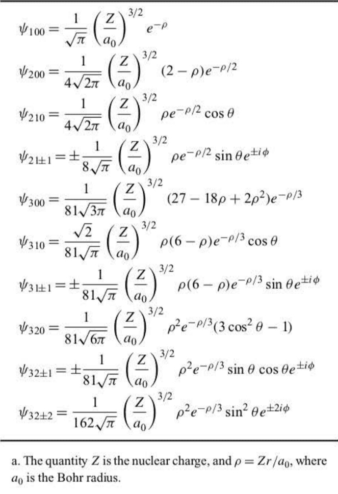
The complete hydrogen atomic wave functions are:

$\psi_{nlm_l}(r,\theta,\phi)=R_{nl}(r)Y_l^{m_l}(\theta,\phi)$

condition for hydrogen atomic wave functions is:

$\langle n\ l\ m_l|n\ l\ m_l \rangle =1 \\[3mm] \langle n\ l\ m_l|n'\ l'\ m_l' \rangle =\delta_{nn'}\delta_{ll'}\delta_{m_lm_l'}$

Note that $\psi_{n\ l\ m_l}(r,\theta,\phi)=|n\ l\ m_l \rangle$ depends upon three quantum numbers. These functions are simultaneous eigenfunctinos of $\hat H$, $\hat L^2$, and $\hat L_z$, which mutually commute:

$[\hat H,\hat L^2]=[\hat H,\hat L_z]=[\hat L^2,\hat L_z]=0$

$n$ for the Hamiltonian operator (the energy), $l$ for the $\hat L^2$ operator (the orbital angular momentum), and $m_l$ for the $\hat L_z$ operator (the z component of the orbital angular momentum) of the commuting set of operators.

Because $\hat H$, $\hat L^2$, and $\hat L_z$ commute with $\hat H$, their corresponding physical observable quantities (energy, orbital angular momentum and its z component) are conserved (see Section 4.9). Their corresponding quantum numbers, $n$, $l$, and $m_l$, which are fixed and so can be used to label the wave function, are said to be good quantum numbers.

（ 与$\hat H$对易，且不依赖时间的算符，其本征值是守恒量。因此，与本征值相对应的量子数就可以用来表征波函数，称为好量子数。 ）

7.2 s Orbitals Are Spherically Symmetric

The hydrogen atomic wave functions depend upon three quantum numbers, $n$, $l$, and $m_l$. The quantum number $n$ is called the principal quantum number and has the values $1,2,\cdots$ The energy of the hydrogen atom depends upon only the principal quantum number through the equation $E_n=-e^2/8\pi\epsilon_0a_0n^2$.

The quantum number $l$ is called the angular-momentum quantum number and has the values $0,1,\cdots,n-1$. The magnitude of the angular momentum of the electron about the proton is determined completely by $l$ through $|L|=\hbar\sqrt {l(l+1)}$.

Note that the form of the radial wave functions depends upon both $n$ and $l$. The value of I is customarily denoted by a letter, with $l=0$ being denoted by $s$, $l=1$ by $p$, $l=2$ by $d$, $l=3$ by $f$. The origin of the letters $s,p,d,f$ is historic and has to do with the designation of the observed spectral lines of atomic sodium. (The letters $s,p,d$ and $f$ stand for sharp, principal, diffuse, and fundamental.)

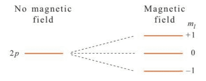
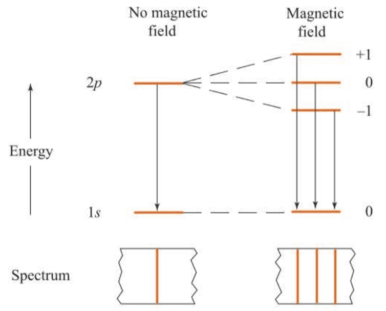
The third quantum number $m_l$ is called the magnetic quantum number and takes on the $2l+1$ values $m_l=0,\pm1,\pm2,\cdots$. The z component of the angular momentum is determined completely by $m_l$ through $L_z=m_l\hbar$. The quantum number $m_l$ is called the magnetic quantum number because the energy of a hydrogen atom in a magnetic field depends on $m_l$. In the absence of a magnetic field, each energy level has a degeneracy of $2l+1$. In the presence of a magnetic field, these levels split, and the energy depends upon the particular value of $m_l$. This splitting is illustrated in Figure 7.2 and is called the Zeeman effect, which is discussed in Section 7.4.

The state of lowest energy of a hydrogen atom is the $1s$ state. The radial function associated with the $1s$ state is:

$R_{1s}(r)=\frac {2}{a_0^{3/2}}e^{-r/a_0}$

For the $1s$ state, the probability that the electron lies between $r$ and $r+dr$ is:

$Prob=r^2R_{1s}^2(r)dr=\frac 4{a_0^3}r^2e^{-2r/a_0}dr$

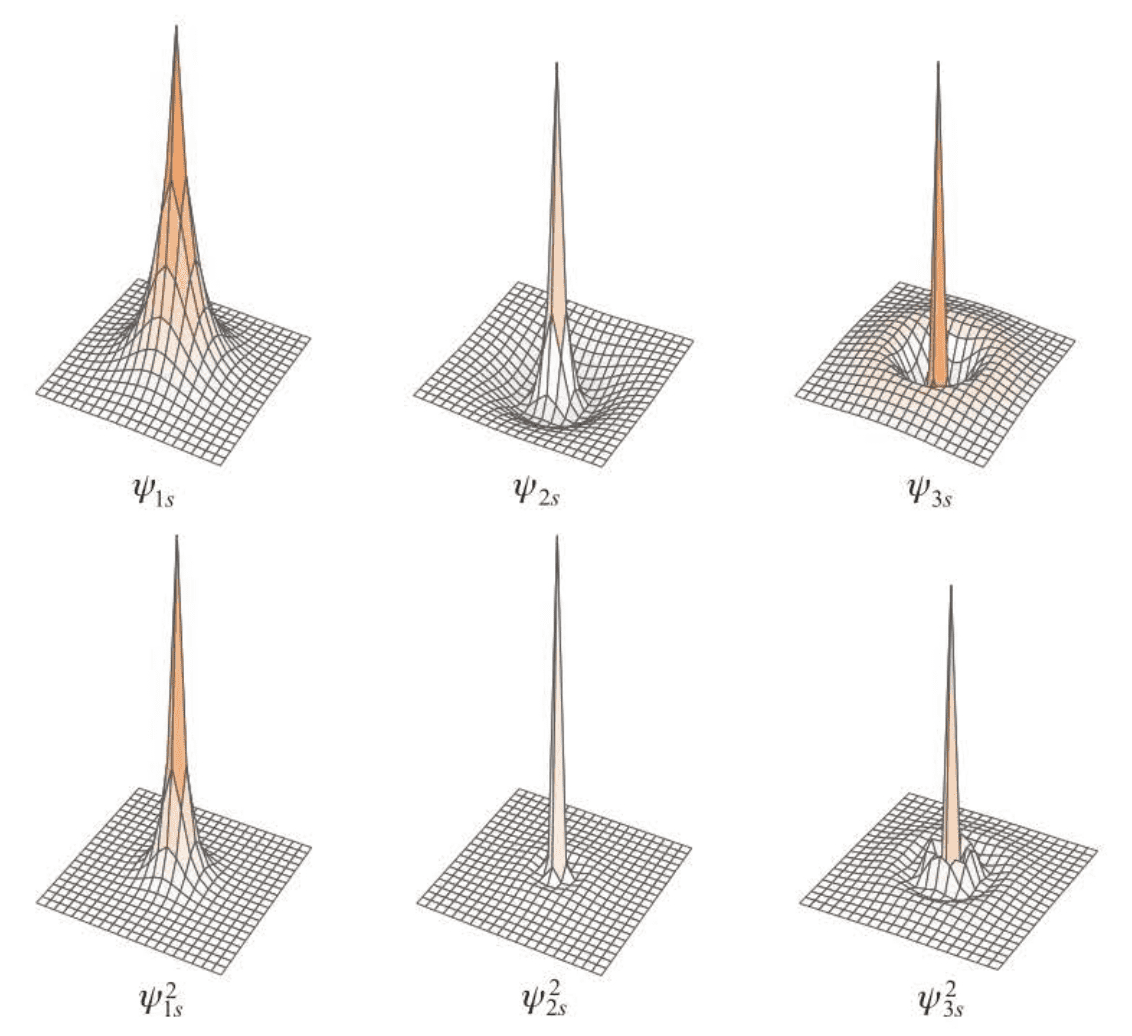
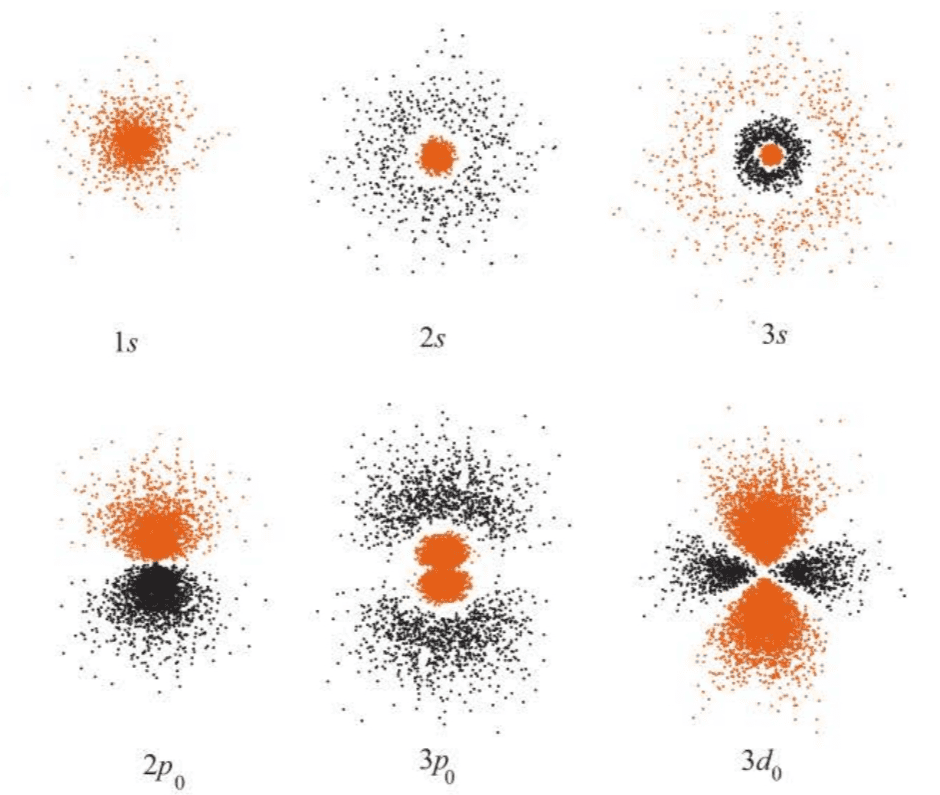
There are more plots of $r^2R_{nl}^2(r)$ shown in Figure 7.3 and surface plots in Figure 7.4.

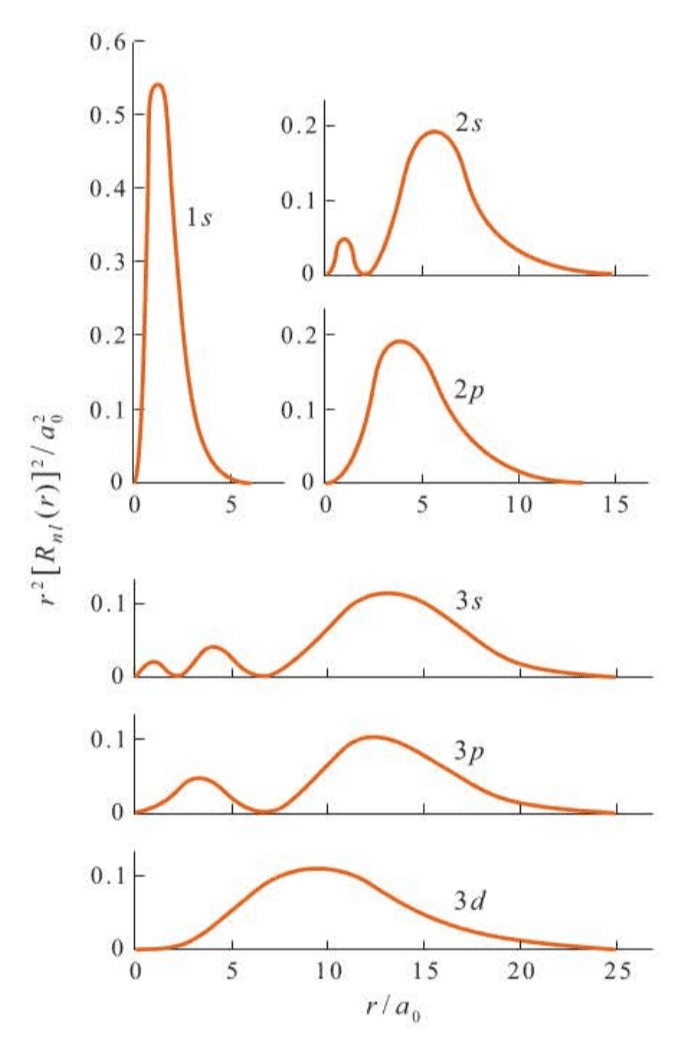
We must keep in mind that we are dealing with only the radial parts of the total wave function here. The radial parts are easy to display because they depend on only the one coordinate, $r$. The angular parts depend on both $\theta$ and $\phi$ and so are somewhat more difficult to display.

The $l=0$ case is easy:

$Y_0^0(\theta,\phi)=\frac 1{\sqrt {4\pi}}$

In this particular case, there is no angular dependence and the wave function is spherically symmetric; in other words, it has the same value for every choice of $(\theta,\phi)$.The complete $1s$ wave function is:

$\psi_{1s}(r,\theta,\phi)=\psi_{100}(r,\theta,\phi)=R_{10}(r)Y_0^0(\theta,\phi)=(\pi a_0^3)^{-1/2}e^{-r/a_0}$

The hydrogen atomic wave functions are called orbitals, and, the equation describes the $1s$ orbital; an electron in the $1s$ state is called a $1s$ electron.

We can calculate the average potential energy in the $1s$ state:

$\langle V(r) \rangle_{1s}=\langle 100|V|100 \rangle =-\frac {e^2}{4\pi\epsilon_0a_0}$

It is interesting to note that $\langle V(r) \rangle=2\langle E \rangle$. Because $\langle T \rangle+\langle V \rangle=\langle E \rangle$ ,where $\langle T \rangle$ is the average kinetic energy, we have $\langle V \rangle=-2\langle T \rangle$, or:

$\frac {\langle V \rangle}{\langle T \rangle}=-2$

It’s generally true for any system in which the potential energy is coulombic. The equation is an example of the virial theorem and is valid for atoms and molecules.

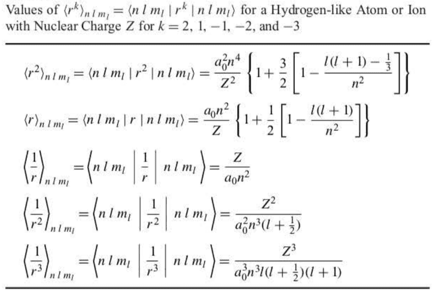
In fact, using the general properties of the radial wave functions, we can show that:

7.3 There Are Three p Orbitals for Each Value of the Principal Quantum Number, $n\ge 2$

When $l\ne 0$, the hydrogen atomic wave functions are not spherically symmetric; they depend on $\theta$ and $\phi$. In this section, we will concentrate on the angular parts of the hydrogen wave functions.

Let’s first consider states with $l=1$, or $p$ orbitals. Because $m_l=0$ or $\pm1$ when $l=1$, there are three $p$ orbitals for each value of $n$.

$Y_1^0(\theta,\phi)=\left(\frac {3}{4\pi} \right)^{1/2}\cos\theta$

A common way to present the angular functions is as three-dimensional figures. Figure 7.6 is the familiar tangent-sphere picture of a p orbital often presented in general chemistry texts. It is not a faithful representation of the shape of a $p_z$ orbital because the radial functions are not included.

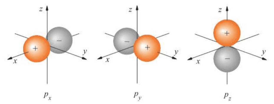
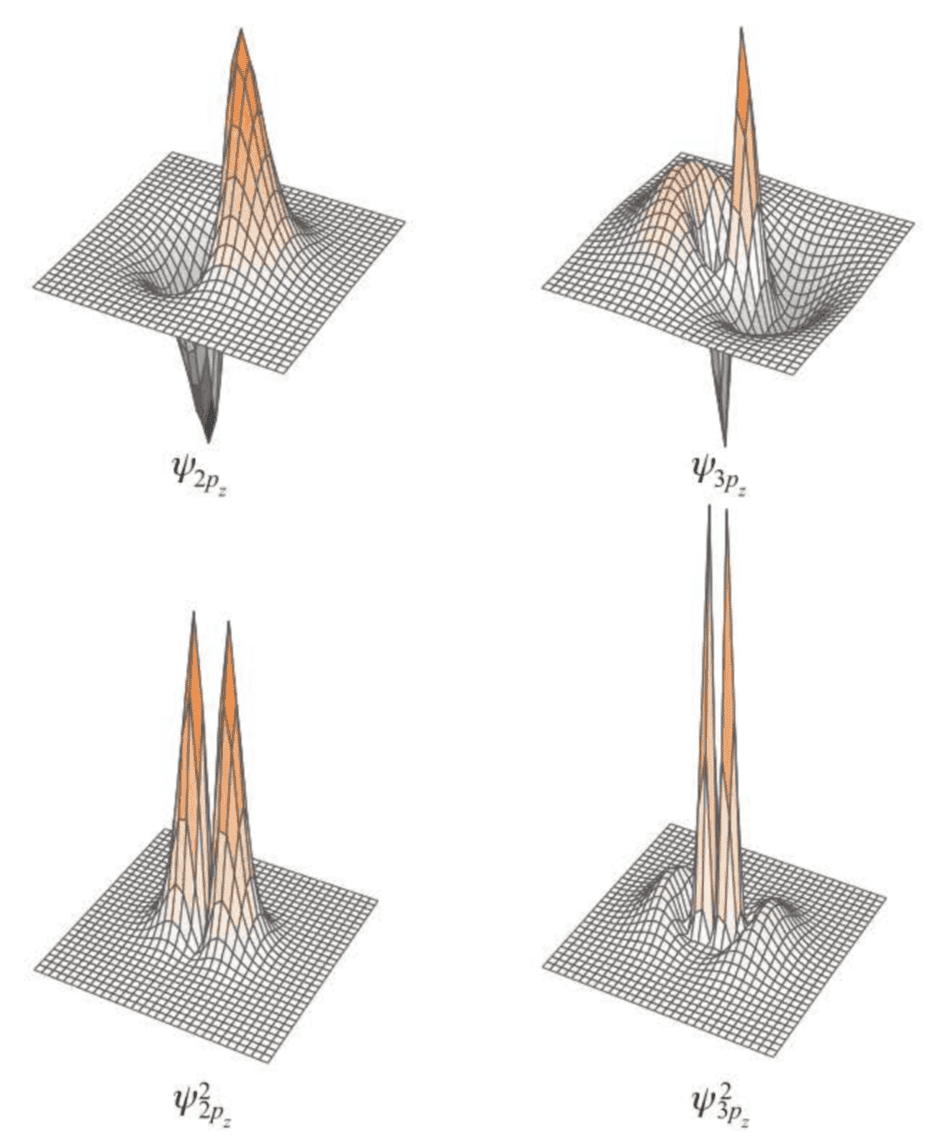
Figure 7.7 shows surface plots of both $\psi_{2p_z}$ and $\psi_{2p_z}^2$ for atomic hydrogen.

An alternate way to represent complete wave functions is as contour maps.

（ 此处介绍了几种绘制波函数的方法，注意图7.6给出的图像仅仅是角度分布图，缺少径向部分的信息，因此严格意义上不是波函数的完整图像。 ）

It is interesting to compare the depictions of the $2p_0$ and $3p_0$ orbitals. Both orbitals have the same angular part. The radial functions have $n-l-1$ nodes, however, and so $R_{21}(r)$ has no nodes and $R_{31}(r)$ has one. This example illustrates the inadequacy of the “tangent-sphere” representation of $p$ orbitals.

The angular functions with $m_l \ne 0$ are more difficult to represent pictorially because they not only depend on $\phi$ in addition to $\theta$, but are complex as well:

$Y_1^{+1}(\theta,\phi)=-\left(\frac 3{8\pi} \right)^{1/2}\sin\theta e^{+i\phi} \\[3mm] Y_1^{-1}(\theta,\phi)=\left(\frac 3{8\pi} \right)^{1/2}\sin\theta e^{-i\phi}$

The probability densities are the same, $|Y_1^{+1}(\theta,\phi)|^2=|Y_1^{-1}(\theta,\phi)|^2$. Because $Y_1^{+1}(\theta,\phi)$ and $Y_1^{-1}(\theta,\phi)$ correspond to the same energy, that any linear combination of $Y_1^{+1}(\theta,\phi)$ and $Y_1^{-1}(\theta,\phi)$ is also an energy eigenfunction with the same energy. It is customary to use the combinations:

$p_x=\frac 1{\sqrt 2}(Y_1^{-1}-Y_1^{+1})=\left(\frac 3{4\pi} \right)^{1/2}\sin\theta \cos\phi \\[3mm] p_y=\frac i{\sqrt 2}(Y_1^{-1}+Y_1^{+1})=\left(\frac 3{4\pi} \right)^{1/2}\sin\theta \sin\phi$

The three functions $p_x,p_y$ and $p_z$ are often used as the angular part of hydrogen atomic wave functions because they are real and have easily visualized directional properties.

（ 当$m_l \ne 0$时，波函数是一个复函数，这在现实世界中是没有意义的，因此通常利用角度函数的线性组合组合出一个实函数，把这个实函数当成波函数的角向部分，利于绘制图像。

类似的，可以继续用线性组合的方法处理$d$轨道并作图，具体过程略去，只展示结果。 ）

$d_{z^2}=Y_2^0=\left(\frac 5{16\pi} \right)^{1/2}(3\cos^2\theta -1) \\[3mm] d_{xz}=\frac 1{\sqrt 2}(Y_2^{-1}-Y_2^{+1})=\left(\frac {15}{4\pi} \right)^{1/2}\sin\theta\cos\theta\cos\phi \\[3mm] d_{yz}=\frac i{\sqrt 2}(Y_2^{-1}+Y_2^{+1})=\left(\frac {15}{4\pi} \right)^{1/2}\sin\theta\cos\theta\sin\phi \\[3mm] d_{x^2-y^2}=\frac 1{\sqrt 2}(Y_2^{+2}+Y_2^{-2})=\left(\frac {15}{16\pi} \right)^{1/2}\sin^2\theta\cos2\phi \\[3mm] d_{xy}=\frac 1{\sqrt 2i}(Y_2^{+2}-Y_2^{-2})=\left(\frac {15}{16\pi} \right)^{1/2}\sin^2\theta\sin2\phi$

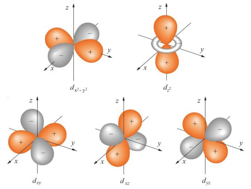
Three-dimensional plots of the angular part of the real representation of the hydrogen atomic wave functions for $l=2$.

7.4 The Energy Levels of a Hydrogen Atom Are Split by a Magnetic Field

In this section, we shall discuss a hydrogen atom in an external magnetic field. We shall see that the magnetic field causes the energy levels to be split into sublevels, which leads to a splitting of the spectral lines in hydrogen. This splitting is called the Zeeman effect.

We shall review some facts and equations concerning magnetic dipoles and magnetic fields:

$\boldsymbol m=\frac {q}{2m}\boldsymbol L$

For an electron, $q=-|e|$:

$\boldsymbol m=-\frac {|e|}{2m_e}\boldsymbol L$

A magnetic dipole will interact with a magnetic field, and the potential energy of a magnetic dipole in a magnetic field is given by:

$V=-\boldsymbol m \cdot \boldsymbol B$

We take the magnetic field to be in the z direction:

$V=-m_zB_z$

With the equation of $m_z$:

$V=\frac {|e|B_z}{2m_e}L_z$

If we replace $L_z$ by its operator equivalent $\hat L_z$, then the equation gives the part of the hydrogen atom Hamiltonian operator that accounts for the external magnetic field. Thus, the Hamiltonian operator for a hydrogen atom in an external magnetic field is:

$\hat H=\hat H_0+\frac {|e|B_z}{2m_e}\hat L_z$

where $\hat H_0$ is the Hamiltonian operator in the absence of a magnetic field.

The corresponding Schrödinger equation is:

$\hat H_0\psi+\frac {|e|B_z}{2m_e}\hat L_z\psi=E\psi$

Therefore, the energy levels of a hydrogen atom in a magnetic field are:

$E=-\frac {m_ee^4}{8\epsilon_0^2h^2n^2}+\beta_Bm_lB_z \quad \left\{\begin{aligned} &n=1,2,3,\cdots \\ &m_l=0,\pm1,\pm2,\cdots,\pm l \end{aligned}\right.$

where $\beta_B$, defined as:

$\beta_B=\frac {|e|\hbar}{2m_e}$

is called a Bohr magneton. Numerically, $\beta_B=9.2740\times10^{-24}J\cdot T^{-1}$.

A state with given values of $n$ and $l$ is split into $2l+1$ levels by an external magnetic field.

The three transitions shown in Figure 7.10 lie very close together, and we say that the $2p\rightarrow1s$ transition becomes a triplet in the presence of an external magnetic field.

（ 当存在外磁场时，系统总能量需要再加上在磁场中的势能，所以能级会进一步分裂，能级分裂项数与$m_l$的取值有关，共$2l+1$项。

不过，上述分析仍存在缺陷，还没有考虑电子自旋产生的影响，实际的光谱线更为复杂，见Section 7.5。 ）

7.5 An Electron Has an Intrinsic Spin Angular Momentum

In 1922, two German physicists, Otto Stern and Walther Gerlach, passed a beam of silver atoms (recall from general chemistry that a silver atom has a $4d^{10}5s^1$ outer electron configuration, and so has a single outer electron) through an inhomogeneous magnetic field in order to split the beam into its $2l+1$ space-quantized components.

Stern and Gerlach found the quite unexpected result that a beam of silver atoms splits into only two parts. Note that this corresponds to $2l+1=2$, or to $l=1/2$. Up to now we have admitted only integer values of $l$.

Another similar observation is the splitting that occurs in atomic spectra. For example, under high resolution it was observed that the $n=2$ to $n=1$ transition in atomic hydrogen is split into two closely spaced lines, called a doublet. These observations cannot be explained using the ideas and equations that we have developed up to now.

In 1925, Wolfgang Pauli showed that all these observations could be explained with the postulate that an electron can exist in two distinct states. Pauli introduced a fourth quantum number in a rather ad hoc manner.

This fourth quantum number, now called the spin quantum number $m_s$, is restricted to the two values $+\frac 12$ and $-\frac 12$. It is interesting that Pauli did not give any interpretation to this fourth quantum number. The existence of a fourth quantum number was somewhat of a mystery because the three spatial coordinates of an electron account for $n$, $l$, and $m_l$, but what is this quantum number due to?

In the early 1930s, the British physicist Paul Dirac developed a relativistic extension of quantum mechanics, and one of its greaitest successes is that spin arose in a perfectly natural way.

We shall introduce spin here, however, in an ad hoc manner.

（ 前面是科学史环节，简单说就是现有的理论无法解释谱线分裂的实验现象，因此波尔提出了自旋磁量子数的概念，但是仍然没有给出合理的理论解释。直到狄拉克提出了狄拉克方程，才从相对论量子力学的角度解释了自旋现象。当然，初等量子力学一般不会讲狄拉克方程。 ）

We define the spin operator $\hat S^2$ and $\hat S_z$ and their eigenfunctions $\alpha$ and $\beta$ by the equations:

$\hat S^2\alpha=\hbar^2s(s+1)\alpha \quad \hat S^2\beta=\hbar^2s(s+1)\beta \quad s=\frac 12 \\[3mm] \hat S_z\alpha=\frac 12\hbar\alpha \quad \hat S_z\beta=-\frac 12\hbar\beta$

We can say that the spin angular momentum of an electron is:

$S=\hbar\sqrt{s(s+1)}$

Unlike $l$, which can vary from 0 to $\infin$, $s$ can have only the value $s=\frac 12$. Note that because $s$ is not allowed to assume large values, the spin angular momentum can never assume classical behavior. Spin is strictly a nonclassical concept. The functions $\alpha$ and $\beta$ are called spin eigenfunctions. We assume that $\alpha$ and $\beta$ are orthonormal, which we write formally as:

$\langle \alpha|\alpha \rangle=\langle \beta|\beta \rangle=1 \\ \langle \alpha|\beta \rangle=\langle \beta|\alpha \rangle=0$

For spin states, $l\rightarrow s=\frac 12$ and $m_l\rightarrow m_s=\pm\frac l2$, we can make the correspondence:

$\alpha =|\frac 12\ \frac 12 \rangle \quad \beta=|\frac 12\ -\frac 12 \rangle$

$\hat S^2|s\ m_s \rangle =\hbar^2s(s+1)|s\ m_s \rangle \quad s=\frac 12 \\[3mm] \hat S_z|s\ m_s \rangle=\hbar m_s|s\ m_s \rangle \quad m_s=\pm\frac 12$

We must now include the spin functions $\alpha$ and $\beta$ with the spatial functions. To a first approximation, the spatial and spin parts of the wave function are independent and so we write:

$\Psi_{n,l,m_l,m_s}(r,\theta,\phi,\sigma)=\psi_{n,l,m_l}(r,\theta,\phi)\alpha(\sigma) \quad or \quad|n\ l\ m_l\ m_s \rangle$

Thus, four quantum numbers are required to specify the state of an electron in a hydrogen atom. The complete one-electron wave function $|n\ l\ m_l\ m_s \rangle$ is called a spin orbital.

（ 自旋是完全量子化的概念，它无法对应经典的性质。尽管不那么直观，我们还是可以用很多物理或数学的方式来描述它。至于自旋到底是什么，只能说它是粒子的一种内禀性质。 ）

7.6 Spin-Orbit Interaction Affects the Energies of a Hydrogen Atom

We saw in Section 7.4 that an electron has a magnetic moment that is proportional to its orbital angular momentum, or that:

$\boldsymbol m_L =-\frac {|e|}{2m_e}\boldsymbol L$

There is also a magnetic moment associated with the spin of the electron. In order to obtain agreement with a number of experimental observations, we must modify the equation by introducing a factor $g$ and write:

$\boldsymbol m_S=-\frac {g|e|}{2m_e}\boldsymbol S$

This Hamiltonian operator yields the energies $E_n=-m_ee^4/8\epsilon_0^2\hbar^2n^2$, which give a very good description of the hydrogen atomic spectrum. Nevertheless, there are discrepancies. For example, a close examination of the $n=2$ to $n=1$ transition shows that it consists of a doublet, which is one of many observations that led Uhlenbeck and Goudsmit to introduce electron spin into quantum mechanics.

It was soon recognized that it was necessary to take into account the fact
that the magnetic moment due to orbital angular momentum and the magnetic moment due to spin angular momentum interact with each other, just as two magnets interact with each other, and the energy of this interaction must be included in the Hamiltonian operator:

$\hat H=-\frac {\hbar^2}{2m_e}\nabla^2-\frac {e^2}{4\pi\epsilon_0r}+\xi(r)\hat {\boldsymbol L}\cdot \hat {\boldsymbol S}$

The added term is called the spin-orbit interaction form.

Realize that spin-orbit interaction is a small effect in a hydrogen atom, and that the resultant energies are going to differ only slightly from the electrostatic energies $E_n=-m_ee^4/8\epsilon_0^2\hbar^2n^2$. We are not able to solve the Schrödinger equation exactly with the spin-orbit interaction term included, but because the effect of the term is small, we expect that the energies $E_n=-m_ee^4/8\epsilon_0^2\hbar^2n^2$ will be altered only slightly by its inclusion. We can use a technique called perturbation theory to calculate how much the electrostatic energies are altered (perturbed).

When the spin-orbit interaction is taken into account, $\hat L^2$ and $\hat S^2$ no longer commute with $\hat H$ and so $\boldsymbol L$ and $\boldsymbol S$ are no longer conserved; only the total angular momentum is conserved:

$\boldsymbol J=\boldsymbol L+\boldsymbol S$

So we have:

$\hat J^2|jm_j\rangle=\hbar^2j(j+1)|jm_j\rangle \quad and \quad \hat J_z|jm_j\rangle =\hbar m_j|jm_j\rangle$

If spin-orbit interaction is considered, then the energy of a hydrogen atom depends upon $n$ and $j$. The general theory to determine $j$ is a little bit involved, but it’s fairly easy to determine the allowed values of $j$ in this case, however, because $s=1/2$ and $m_s$ can assume only two values, $\pm1/2$.

There are $2l+1$ possible orbital angular-momentum states for a fixed value of $l$ and $2s+1=2$ possible spin angular-momentum states, giving $2(2l+1)$ as the total number of states.

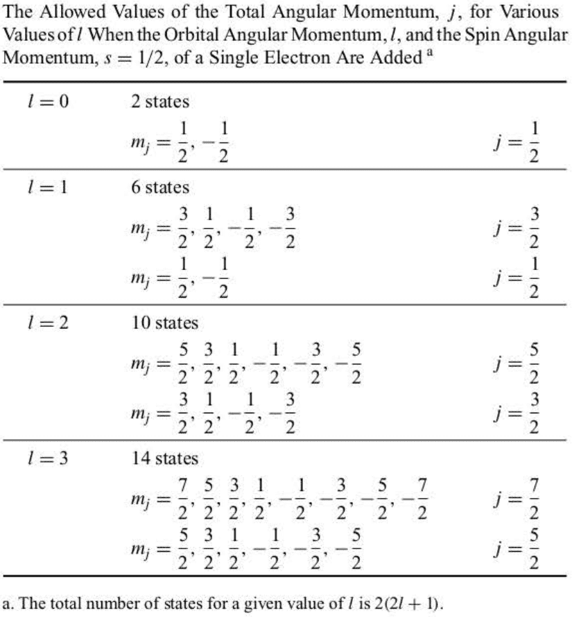
We can summarize all these results in one equation by writing:

$j=l+s \quad and \quad |l-s|$

When $l=0$, we have $j=1/2$; when $l=1$, we have $j=3/2$ and $1/2$; and when $l=2$, we have $j=5/2$ and $3/2$, and so on.

7.7 The Electronic Energy Levels of a Hydrogen Atom Are Described by Term Symbols

We designate the electronic states of a hydrogen atom by an atomic term
symbol, which is expressed by the occupied orbital followed by the symbol $^2l_j$. The left superscript here represents the multiplicity (degeneracy) of the spin, which is $2s+1=2$. In writing a term symbol for atomic hydrogen, we make the correspondence:

$\begin{aligned}l=\ &0\quad\ 1\quad\ 2\quad\ 3\quad\ 4 \\ &S\quad P\quad D\quad F\quad G \quad etc. \end{aligned}$

Therefore, the ground electronic state, for which $l=0$ and $j=1/2$, is designated by $1s\ ^2S_{1/2}$.

Let’s look at the Lyman series, which is the series of lines that arise from transitions from states with $n\ge2$ to the $n=1$ state. We can use the Rydberg formula to calculate the frequencies of the lines in the Lyman series:

$\tilde \nu =109\,677.58 \left(1-\frac 1{n^2} \right)cm^{-1} \quad n=2,3,\cdots$

Not all these states can make a transition to the ground state because of selection rules. Recall that selection rules are restrictions that govern the possible, or allowed, transitions from one state to another. In the case of atomic spectra, the selection rules are:

$\Delta L =\pm1 \\ \Delta S=0 \\ \Delta J=0,\pm1$

except that a transition from a state with $J=0$ to another state with $J=0$ is not allowed (forbidden). Thus, if we look closely at the Lyman series of atomic hydrogen, we see that the allowed transitions into the ground state are:

$np\ ^2P_{1/2} \rightarrow 1s\ ^2S_{1/2}$

or

$np\ ^2P_{3/2} \rightarrow 1s\ ^2S_{1/2}$

No other transitions into the $1s\ ^2S_{1/2}$ ground state are allowed.

Atomic term symbols are sometimes called spectroscopic term symbols because atomic spectral lines can be assigned to transitions between states that are described by atomic term symbols.

The values of the frequencies associated with the $2\rightarrow 1$ transitions can be computed:

$\tilde \nu = 82\,258.9206 cm^{-1} \\ \tilde \nu= 82\,259.2865 cm^{-1}$

This closely spaced pair of lines is called a doublet, and so we see that under high resolution, the first line of the Lyman series is a doublet. We find that all the lines of the Lyman series are doublets and that the separation of the doublet lines decreases with increasing $n$. The increased spectral complexity caused by spin-orbit coupling is called fine structure.

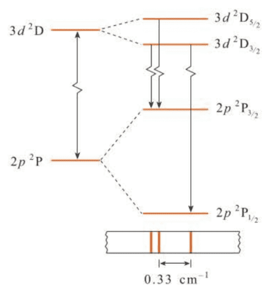
（ 在考虑自旋-轨道耦合之后，可以进一步解释谱线的分裂现象，即光谱的精细结构。 ）

7.8 The Spectrum of Atomic Hydrogen in an External Magnetic Field Is Accounted for by the Zeeman Effect

We predicted at that time that the $2p \rightarrow 1s$ transition should be split into three lines, which is not in accord with experiment. In fact, ten lines are
observed. We claimed that this discrepancy is due to the spin of the electron, and in this section, we shall see how these ten lines arise.

The total magnetic moment is $\boldsymbol m_L+\boldsymbol m_S$, and the energy of its interaction
with an external magnetic field (which is taken to be in the z direction) is given by:

$V=\frac {|e|B_z}{2m_e}(L_z+gS_z)$

For typical magnetic field strengths, the effect of $V$ is small and can be treated by perturbation theory. The final result is that the states are split by:

$\Delta E_{mag}=g(j,l)\beta_Bm_jB_z$

where $m_j=-j,-j+1,\cdots,0,1,\cdots,+j$ and:

$g(j,l)=\left\{\begin{aligned} 2\left(\frac {l+1}{2l+1}\right) \quad j=l+\frac 12 \\[3mm] \frac {2l}{2l+1} \quad j=l-\frac 12 \end{aligned}\right.$

This quantity $g(j,l)$ is known as the L****andé g factor. Note that $g=2$ for the $1s\ ^2S_{1/2}$ states, $2/3$ for the $2p\ ^2P_{1/2}$ states, and $4/3$ for the $2p\ ^2P_{3/2}$ states.

Figure 7.13 shows the splitting of the $1s\ ^2S_{1/2}$, $2p\ ^2P_{1/2}$ and $2p\ ^2P_{3/2}$ states in an external magnetic field. The allowed transitions ($\Delta m_j=0,\pm1$) are indicated, along with a schematic sketch of the resulting spectrum. Note that there are ten lines in the $2p \rightarrow 1s$ transition.

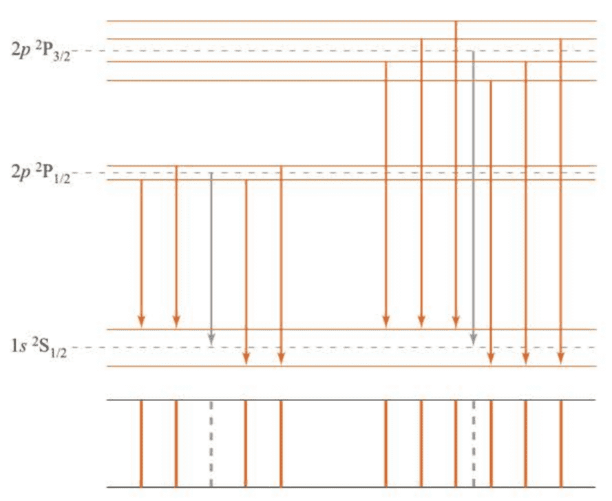
（ 在考虑了自旋-轨道耦合之后，谱线进一步分裂，满足选律的能级跃迁所产生的谱线共有10条。 ）

7.9 The Schrödinger Equation for a Helium Atom Cannot Be Solved Exactly

The next system to study is the helium atom, whose Schrödinger equation is:

$\left(-\frac {\hbar^2}{2M}\nabla^2-\frac {\hbar^2}{2m_e}\nabla_1^2-\frac {\hbar^2}{2m_e}\nabla_2^2 \right)\psi(\boldsymbol R,\boldsymbol r_1,\boldsymbol r_2)+\left(-\frac {2e^2}{4\pi\epsilon_0|\boldsymbol R-\boldsymbol r_1|}-\frac {2e^2}{4\pi\epsilon_0|\boldsymbol R-\boldsymbol r_2|}+\frac {e^2}{4\pi\epsilon_0|\boldsymbol r_1-\boldsymbol r_2|} \right)\psi(\boldsymbol R,\boldsymbol r_1,\boldsymbol r_2)=E\psi(\boldsymbol R,\boldsymbol r_1,\boldsymbol r_2)$

In this equation, $\boldsymbol R$ is the position of the helium nucleus, and $\boldsymbol r_1$ and $\boldsymbol r_2$ are the positions of the two electrons; $M$ is the mass of the nucleus, and $m_e$ is the electronic mass; $\nabla^2$ is the Laplacian operator with respect to the position of the nucleus, and $\nabla_1^2$ and $\nabla_2^2$ are the Laplacian operators with respect to the positions of the electronic coordinates.

Realize that this is a three-body problem and not a two-body problem, and so the separation into center-of-mass and relative coordinates is much more complicated than it is for hydrogen.

Because $M \gg m_e$, however, regarding the nucleus as fixed relative to the
motion of the electrons is still an excellent approximation:

$-\frac {\hbar^2}{2m_e}\left(\nabla^2_1+\nabla_2^2\right)\psi(\boldsymbol r_1,\boldsymbol r_2) - \frac {2e^2}{4\pi\epsilon_0}\left(\frac 1{r_1}+\frac 1{r_2} \right)\psi(\boldsymbol r_1,\boldsymbol r_2) + \frac {e^2}{4\pi\epsilon_0|\boldsymbol r_1 - \boldsymbol r_2|}\psi(\boldsymbol r_1,\boldsymbol r_2)=E\psi(\boldsymbol r_1,\boldsymbol r_2)$

Even this simplified equation cannot be solved exactly.

Because we cannot solve the equation exactly, we must resort to some approximation method. Fortunately, two quite different approximation methods that can yield extremely good results have found wide use in quantum chemistry. These are called the variational method and perturbation theory and are presented in the next chapter.

总结

本章的内容可以说是结构化学/量子化学老生常谈的部分了，很多结论在无机化学中也都很熟悉，另外还涉及了一些光谱学的内容。